We give a novel approach to proving soundness and completeness for a logic (henceforth: the object-logic) that bypasses truth-in-a-model to work directly with validity. Instead of working with specific worlds in specific models, we reason with eigenworlds (i.e., generic representatives of worlds) in an arbitrary model. This reasoning is captured by a sequent calculus for a meta-logic (in this case, first-order classical logic) expressive enough to capture the semantics of the object-logic. Essentially, one has a calculus of validity for the object-logic. The method proceeds through the perspective of reductive logic (as opposed to the more traditional paradigm of deductive logic), using the space of reductions as a medium for showing the behavioural equivalence of reduction in the sequent calculus for the object-logic and in the validity calculus. Rather than study the technique in general, we illustrate it for the logic of Bunched Implications (BI), thus IPL and MILL (without negation) are also treated. Intuitively, BI is the free combination of intuitionistic propositional logic and multiplicative intuitionistic linear logic, which renders its meta-theory is quite complex. The literature on BI contains many similar, but ultimately different, algebraic structures and satisfaction relations that either capture only fragments of the logic (albeit large ones) or have complex clauses for certain connectives (e.g., Beth’s clause for disjunction instead of Kripke’s). It is this complexity that motivates us to use BI as a case-study for this approach to semantics.
1 Introduction
This paper centres around a new approach for proving soundness and completeness.
It is an extended case-study of the method applied to the logic of Bunched Implications (BI) [24], which is chosen as the subject because the complexities in the logic’s syntax and meta-theory help expose the more subtle aspects of how and why the method works. Essentially, the approach proceeds by showing extensional equivalence of the provability and validity judgments by showing behavioural equivalence of transition systems (i.e., reduction in sequent calculi—see below) for them. This supports the intuition that rules for the connectives in a proof system define their meaning, the central doctrine to proof-theoretic semantics [30], since it is with the rules of the sequent calculus that the clauses of satisfaction must match in order to witness soundness and completeness.
A distinguishing feature of BI is that it contains two primitive variants of conjunction and implication, one additive and one multiplicative. Consequently, contexts in BI are not lists, multisets, nor sets, they are instead bunches, a data-structure constructed out of formulas using two contextformers, one for each conjunction. Individually, the context-formers behave as expected (i.e., they are commutative and associative), but they do not commute with each other. The interaction between the additive and multiplicative parts of the logic renders much of the meta-theory of BI subtle and complex. In this paper, the a priori characterization of BI is provided by the logic’s sequent calculus LBI [2,26]. The choice of the sequent calculus over the other formalisms available for BI (e.g., Hilbert or natural deduction systems) is because the space of derivations is simpler to characterize than in other systems. Firstly, using a proof system over sequents means that all of the data during any stage of a derivation is contained locally. Secondly, the sequent calculus has the advantage over the sequent presentation of natural deduction in that its reductions are simpler to characterize because of its proof-theoretic features (e.g., the sub-formula property). A sequent is a pair $\Gamma \rhd \varphi$ in which $\Gamma$ is a bunch, called the context, and $\varphi$ is a formula, called the extract. The nomenclature is purposefully suggestive: the context is regarded as available information, and the extract as inferred information. Yet, sequents are unjudged structures.
A sequent $\Gamma \rhd \varphi$ is a consequence of BI when it has a proof in LBI.
This paper concerns the model theory of BI. One gives a model-theoretic account of BI by means of a satisfaction relation of the form $w \Vdash \varphi$, in which the possible worlds w are elements from a structure called a frame, and the $\varphi$ are formulas. A sequent $\Gamma \rhd \varphi$ is valid if, in any model $\mathfrak{M}$, at any world w in that model, if $w \Vdash \Gamma$, then $w \Vdash \varphi$. We write $\Gamma \vDash \varphi$ to denote that $\Gamma \rhd \varphi$ is valid. In this paper, we show the soundness and completeness of BI with respect to the (putative) semantics—provability is sound with respect to validity when $\Gamma \vdash \varphi$ implies $\Gamma \vDash \varphi$; provability is complete when $\Gamma \vDash \varphi$ implies $\Gamma \vdash \varphi$. From this perspective, one expects the proof-theoretic and modeltheoretic views of logic to be reasonably close.
Various sound and complete semantics have been studied for BI in the past, including categorical, relational, and topological variants (specially, Grothendieck topological semantics close the Hilbert calculi for BI—see Pym [25]), but the most widely used models of BI in the literature employ the monoidal semantics, for which completeness has been a subtle problem. Currently, soundness and completeness results have been achieved only for monoids with partial or non-deterministic products or with total deterministic products but with Beth’s clause for disjunction in the definition of satisfaction. These previous results are discussed in Section 6. In this paper, we prove completeness for a general class of relational models, which subsumes the relational and monoidal semantics discussed above, while employing Kripke’s clause for disjunction. That this is possible while avoiding the complications that arise in previously considered term-model constructions demonstrates the strength of the approach.
The intuition behind the approach to soundness and completeness in this paper is that the ways in which proof theory and model theory define the connectives coincide; for example, in both paradigms, additive conjunction is characterized by the behaviour that relative to some available information $\Gamma$ one has the conjunction $\varphi \land \psi$ if and only if, relative to the same information, one has each of $\varphi$ and $\psi,$ independently. Essentially, the approach in this paper proceeds by showing that whatever reasoning can be done in the model theory can be simulated in the model proof theory, and vice versa. We characterize reasoning through the perspective on logic called reductive logic— dual to the more traditional paradigm of deductive logic— as explorations of the space of reductions in a sequent calculus.
A formal definition of the space of reductions is contained within (see Section 3), but it is only a formal treatment of the intuitive idea as the space of derivations accessible by means of reductive reasoning (i.e., by using sequent calculus rules backward) from a given sequent.
To characterize validity in terms of a space of reductions, one needs a proof system for it, which is handled by encoding it with a meta-logic (firstorder classical logic) such that worlds and formulas become terms and satisfaction becomes a relation symbol. This is similar to other uses of logic to reason about mathematical objects and structures (e.g., the use of logic in universal algebra and applied logic); see Section 4.1 for more discussion. Therefore, the central part of the paper concerns giving a sequent calculus for a restriction of the meta-logic expressive enough to reason about validity, while tractable enough to characterize its space of reduction. Since we work with eigenvariables representing worlds, dubbed eigenworlds, we bypass truth-in-a-model. In particular, the reasoning being witnessed in the meta-logic can be instantiated to any world in any model.
The paper begins in Section 2 with a terse, but complete, proof-theoretic and semantic formulation of BI; it continues in Section 3 with a brief summary of the space of reductions for a sequent in a sequent calculus. This background is followed in Section 4 by an analysis of model-theoretic reasoning as captured by reduction in a meta-logic. The main result of the paper is in Section 5, where we prove soundness and completeness using behavioural equivalence of reductions in the sequent calculus and in the semantics (i.e., in a sequent calculus for the meta-logic capturing validity). In Section 6, we discuss the literature on the semantics of BI and contrast the major result with the work of this paper; more specifically, in Section 7, we review Beth’s clause for disjunction in this context. The paper concludes in Section 8 with a summary of the main theorem and thesis, and a proposal of future work.
2 The Logic of Bunched Implications
In this section, we give a syntactic and proof-theoretic account of BI that provides the concept of BI-truth, as well as define the concept of a model for which we prove soundness and completeness. Specifically, Section 2.1 recalls the usual sequent calculus for BI, Section 2.2 provides the proof theory used in this paper, and Section 2.3 introduces the (putative) model theory.
2.1 Syntax
The logic of Bunched Implications (BI) [24] can be regarded as the free combination (i.e., the fibration—see Gabbay [12]) of (additive) intuitionistic logic, with connectives $\land,\lor,\to,\top,\bot$, and multiplicative intuitionistic logic, with connectives $\ast$, $\wand$, $\top^*$. A distinguishing feature of BI is that contexts are not one of the familiar structures of lists, multisets, or sets, since the two context-formers $\rsemi$ and $\rcomma$, representing the two conjunctions $\land$ and $\ast$, respectively, do not commute with each other, though individually they behave as usual; contexts are instead bunches—a term that derives from the relevance logic literature (see, for example, Read [28]).
Let P be a set of propositional letters. The set of formulas F is defined by the following grammar: $$\varphi ::= p \in \mathbb{P} \mid \top \mid \bot \mid \top^* \mid \varphi \land \psi \mid \varphi \lor \psi \mid \varphi \to \varphi \mid \varphi \ast \varphi \mid \varphi \wand \varphi$$
The set of bunches B is defined by the following: $$\Gamma ::= \varphi \in F \mid \emptyset_+ \mid \emptyset_\times \mid \Gamma \rsemi \Gamma \mid \Gamma \rcomma \Gamma$$ The $\rsemi$ is the additive context-former, and the $\emptyset_+$ is the additive unit; the $\rcomma$ is the multiplicative context-former, and the $\emptyset_\times$ is the multiplicative unit.
A BI-sequent is a pair $\Gamma \rhd \varphi$ in which $\Gamma$ is a bunch, called the context, and $\varphi$ is a formula, called the extract. The empty pair, denoted $\Box$, is also a sequent. A sub-tree $\Delta$ of a bunch $\Gamma$ is a sub-bunch. We may write $\Gamma(\Delta)$ to express that $\Delta$ is a sub-bunch of $\Gamma$. The operation $\Gamma[\Delta \to \Delta']$—abbreviated to $\Gamma(\Delta')$, where no confusion arises—is the result of replacing the occurrence of $\Delta$ by $\Delta'$. Since contexts are more complex than in many of the more familiar logics (e.g., classical logic, intuitionistic logic, etc), the following is an explicit characterization of the analogous structural behaviour (i.e., equivalence upto permutation):
Two bunches $\Gamma, \Gamma' \in \mathbb{B}$ are coherently equivalent when $\Gamma \equiv \Gamma'$, where $\equiv$ is the least relation satisfying:
– commutative monoid equations for $\rsemi$ with unit $\emptyset_+$;
– commutative monoid equations for $\rcomma$ with unit $\emptyset_\times$;
– coherence; that is, if $\Delta \equiv \Delta'$ then $\Gamma(\Delta) \equiv \Gamma(\Delta')$. Bunches are typically understood as the syntax trees provided by Definition 2.2 modulo coherent equivalence, in the same way that lists for the contexts of classical logic sequents are understood modulo permutation. The idea that the context-formers represent the conjunctions provides the following transformation:
The compacting function $\lfloor - \rfloor : \mathbb{B} \to \mathbb{F}$ is fixed on formulas—that is, $\lfloor \varphi \rfloor := \varphi$—and acts on non-formulas as follows: $$\lfloor \Gamma \rcomma \Delta \rfloor := \lfloor \Gamma \rfloor \ast \lfloor \Delta \rfloor \quad \lfloor \emptyset_\times \rfloor := \top^* \quad \lfloor \Gamma \rsemi \Delta \rfloor := \lfloor \Gamma \rfloor \land \lfloor \Delta \rfloor \quad \lfloor \emptyset_+ \rfloor := \top$$
That a sequent $\Gamma \rhd \varphi$ is a consequence of BI is denoted $\Gamma \vdash \varphi$. In this paper, the a priori characterization of consequence is through provability, which is the subject of the next section.
2.2 Proof Theory
In this paper, we use various structures that we call sequent (i.e., not just BIsequent). For each such structure, we will require the same general notions of rule and proof. Therefore, for the sake of economy, the definitions below apply to any fixed notion of sequent.
A rule r is a relation on sequents. The situation $r(S, S_1, \ldots, S_n)$ may be denoted in the following format: $$\dfrac{S_1 \quad \ldots \quad S_n}{S}\ r$$
A sequent calculus is a set of rules. Since much of subsequent work concerns reduction, we define proofs by a correctness criterion rather than the familiar inductive construction (see, for example, Troelstra and Schwichtenberg [32]), doubtless already familiar.
Let L be a sequent calculus and let S be a sequent. A rooted finite tree D of sequents is a L-proof of S, if for any node $\zeta$,
– if $\zeta$ is a leaf, then $\zeta = \Box$;
– if $\zeta$ has children $P_0, \ldots, P_n$ in D, then there is a rule $r \in L$ such that $r(\zeta, P_0, \ldots, P_n)$;
– if $\zeta$ is the root, then $\zeta$ is S. A sequent $\Sigma \rhd \Pi$ is L-provable—denoted $\Sigma \vdash_L \Pi$—if and only if there is an L-proof with root $\Sigma \rhd \Pi$. In this paper, we define consequence for BI ($\vDash$) by provability in the sequent calculus LBI.
System LBI comprises the rules in Figure 1. We use $\Box$ in the premiss of axioms to facilitate the transition between the concept of a proof and the concept of a reduction in a space of reductions in Section 3. Though unusual in much of proof theory, this notation is standard when working with reductions—see, for example, Kowalski [18]. In the remainder of this section, we give some technical results to facilitate subsequent discussion.
For any $\Gamma \in \mathbb{B}$ the following holds: $\Gamma \vdash_{\mathrm{LBI}} \lfloor \Gamma \rfloor$.
This follows from induction on the size of $\Gamma$—see, for example, Gheorghiu and Marin [16].
□The following rules are admissible for BI: $$\dfrac{}{\Gamma \rsemi \varphi \rhd \varphi}\ \text{taut} \qquad \dfrac{\Delta \vdash \varphi \quad \Delta' \rhd \psi}{\Gamma \rsemi (\Delta \rcomma \Delta') \rhd \varphi \ast \psi}\ \ast\mathrm{R} \qquad \dfrac{\Delta \rhd \varphi \quad \Gamma(\varphi) \rhd \chi}{\Gamma(\Delta) \rhd \chi}\ \text{cut}$$
The first two rules are admissible by combining w with Lemma 2.10 and ∗R in Figure 1, respectively. The admissibility of cut was proved by Brotherston [2] (see also Gheorghiu and Marin [16]).
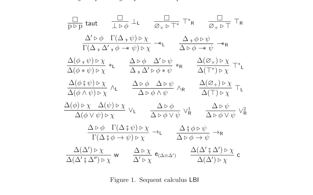
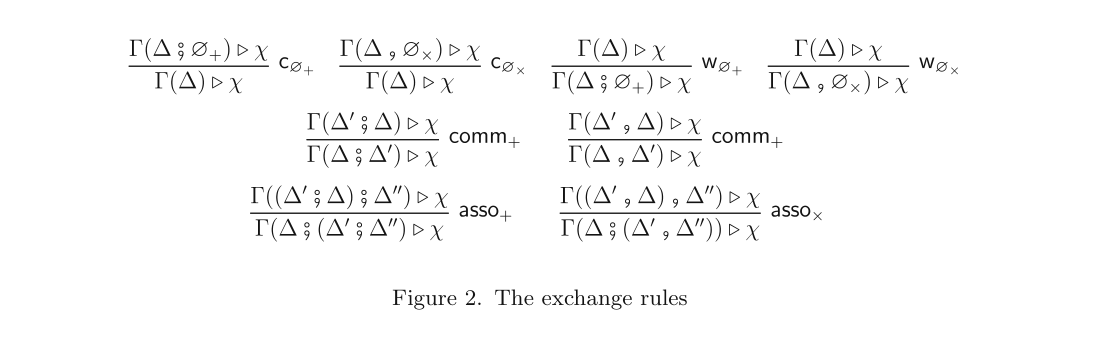
We have overloaded the names taut and ∗R to economize on notation. Henceforth, the names refer to the rules in Lemma 2.11. The underlying ideology in this paper is that the rules of the sequent calculus define the connectives (and context-formers) of the logic. From this perspective, the exchange rule e is not tractable since its definition outsources the key behaviour of the syntax that it concerns. Therefore, we desire a representation of it that is internal to the sequent calculus.
□The rules in Figure 2 are admissible for BI and they have the same expressive power as e.
Since $\Gamma \equiv \Gamma'$ if and only if there is a sequence of steps using the commutative monoid axioms and all of these are encoded by the new rules of Figure 2, these rules are admissible. Taking all these technical results result provides a new sequent calculus for BI suitable for the work in this paper.
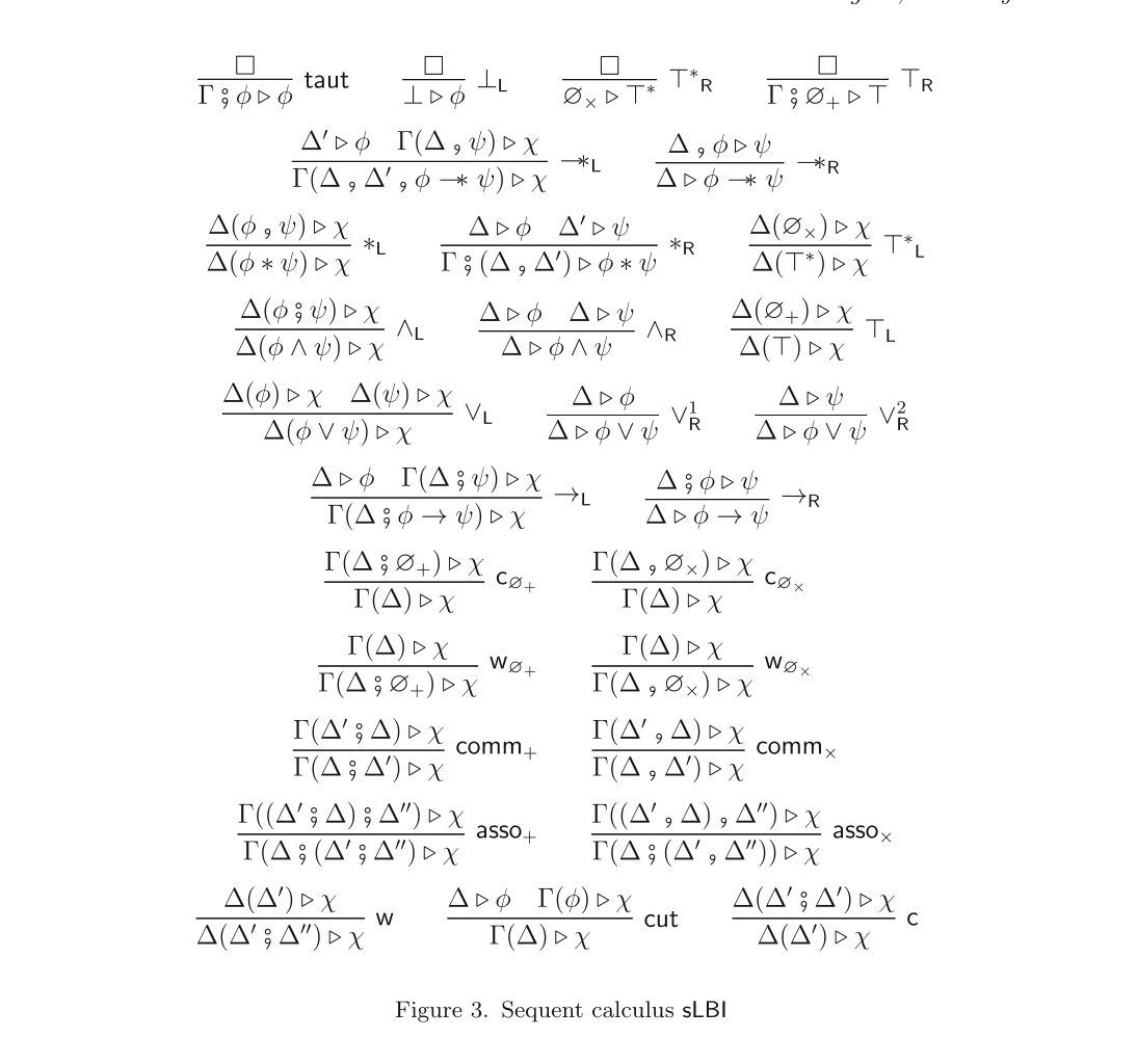
□System sLBI is composed of the rules in Figure 3 in which asso is invertible.
$\Gamma \vdash_{\mathrm{LBI}} \varphi$ iff $\Gamma \vdash_{\mathrm{sLBI}} \varphi$.
2.3 Model Theory
In contrast to classical logic, in the model theory for non-classical logics, one thinks of statements (i.e., formulas of the logic) not as being universally true, but instead true with respect to a certain state of affairs, such as at a certain time or with respect to some information. For intuitionistic propositional logic (IPL), a formula is true when one can provide a method for witnessing (or constructing) it; the states in the model-theoretic semantics for IPL are sometimes understood as witnesses of these methods, and the clauses of the satisfaction relation specify how the witnesses relate to each other—see, for example, Dummett [11] for details. The model-theoretic semantics of BI is an extension of the model-theoretic semantics for IPL that allows witnesses to be decomposed. Decomposition is witnessed by a relation R such that w decomposes to u and v iff R(w, u, v). A witness w satisfies an additive conjunction $\varphi\land\psi$ when it satisfies both $\varphi$ and $\psi,$ and a witness w satisfies a multiplicative conjunction $\varphi \ast \psi$ when there are two states u and v such that R(w, u, v), u satisfies $\varphi,$ and v satisfies $\psi.$ This handling of the semantics is in the style of the style of Routley and Meyer [29] and Urquhart [33] for relevant logics.
A quintuple $\mathfrak{M} := \langle \mathbb{V}, e, \pi, \preceq, R\rangle$ is a BI-frame when $\mathbb{V}$ is a set, e and $\pi$ are distinguished element of the set, $\preceq$ is a preorder on the set dominated by $\pi$—that is, for any w in the set, $w \preceq \pi$—and R is a ternary relation on the set satisfying the following conditions: –(Unitality) R(w, w, e) –(Commutativity) R(x, y, z) iff R(x, z, y) –(Associativity) if R(x, w, y) and R(y, u, v), then there exists a z such that R(x, z, v) and R(z, w, u) The elements of $\mathbb{V}$ in a BI-frame are called worlds.
Let $\mathfrak{F} := \langle \mathbb{V}, e, \pi, \preceq, R\rangle$ be a BI-frame. A mapping $\llbracket-\rrbracket : \mathbb{V} \to \wp(\mathbb{P})$ is an interpretation,
Satisfaction for a pair $\langle \mathfrak{F}, \llbracket-\rrbracket\rangle$ is a binary relation $\Vdash$ between worlds and the formulas, defined by the clauses in Figure 4. We require the following (general) persistence condition on satisfaction, to model BI: $$\text{for any } \varphi \in \mathbb{F} \text{ and any } w, u \in \mathbb{V}, \text{ if } w \preceq u \text{ and } w \Vdash \varphi, \text{ then } u \Vdash \varphi$$
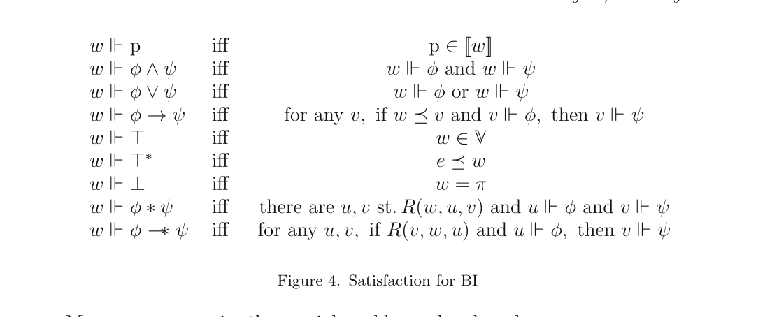
Moreover, we require the special world $\pi$ to be absurd: $$\text{for any } \varphi \in \mathbb{F}, \text{ if there is a world } w \text{ such that } w \Vdash \varphi, \text{ then } \pi \Vdash \varphi$$ This concept of a model given in Definition 2.18 actually arises from the approach to completeness that this paper demonstrates in that the clauses are designed to reflect the proof-theoretic behaviour of the connectives.
A pair $\mathfrak{M} := \langle \mathfrak{F}, \llbracket-\rrbracket\rangle$, in which $\mathfrak{F}$ is a frame and $\llbracket-\rrbracket$ is an interpretation, is a model when it is persistent and, for any $\varphi \in \mathbb{F}$, $\pi \Vdash \varphi$. The set of all models is $\mathcal{C}$. This definition of a frame for modelling BI based on a relation R is more general than that studied by Galmiche et al. [14], whose relationship to the present structure is discussed in Section 6. Similar models to the present one have previously been studied by Docherty and Pym [5,8,10]. In that work, certain variations of satisfaction are also considered that may also be understood from the approach to completeness in this paper, but they are more complex without being more informative for our purposes. In terms of constructing models, the most difficult requirement to satisfy is persistence, but the aforementioned authors have also given conditions under which this condition can be met. A necessary condition is bifunctoriality: $$\text{if } u \preceq u',\ v \preceq v',\ R(w, u, v) \text{ and } R(w', u', v'), \text{ then } w \preceq w'$$ These concerns are discussed further in Section 6.4
A sequent $\Gamma \rhd \varphi$ is valid—denoted $\Gamma \vDash \varphi$—if, for any model $\mathfrak{M} \in \mathcal{C}$, at any world w, if $w \Vdash \Gamma$, then $w \Vdash \varphi$. The intuition for why BI is complete for this class of frames (i.e., $\Gamma \vDash \varphi$ implies $\Gamma \vdash \varphi$) is that it has precisely the structure required to simulate BI in the context-extract reading. The strength of universal quantification on frames and on worlds for $\Gamma \vDash \varphi$ is deceptive since one must show that if $w \Vdash \Gamma$, then $w \Vdash \varphi$, which has more to do with the relationship between $\Gamma$ and $\varphi$ (according to satisfaction) than it does with the frame or with the world.
3 Reductive Logic
The traditional paradigm of logic proceeds by inferring a conclusion from established premisses using an inference rule. This is the paradigm known as deductive logic: $$\dfrac{\text{Established Premiss}_1 \quad \ldots \quad \text{Established Premiss}_n}{\text{Conclusion}}\ \Downarrow$$ In contrast, the experience of the use of logic is often dual to deductive logic in the sense that it proceeds from a putative conclusion to a collection of premisses that suffice for the conclusion. This is the paradigm known as reductive logic: $$\dfrac{\text{Sufficient Premiss}_1 \quad \ldots \quad \text{Sufficient Premiss}_n}{\text{Putative Conclusion}}\ \Uparrow$$ Rules used backward in this way are called reduction operators. The objects created using reduction operators are called reductions.
Historically, the deductive paradigm has dominated since it exactly captures the meaning of truth relative to some set of axioms and inference rules, and therefore is the natural point of view when considering foundations of mathematics. However, it is the reductive paradigm from which much of computational logic derives, including various instances of automated reasoning—see, for example, Kowalski [19], Bundy [3], and Milner [22]. In this paper, reductive logic is the paradigm we use to understand the reasoning used to establish the validity of a BI-sequent. There are many ways of studying reduction, and a number of models have been considered, especially in the case of classical and intuitionistic logic (see, for example, Pym and Ritter [27]). A generic approach to representing and understanding the structure of the space of reductions is the use of coinductive derivations trees, which have their origin in Kowalski’s study of logic programming [18]. A (co-)algebraic treatment has been considered by the authors previously [15], generalizing earlier work by Komandantskaya et al. [17].
Let S be a set of sequents and let L be a sequent calculus over these sequents. For any rule $r \in L$, its reduction operator $\rhoL : S \to \wp\wp(S)$ is the map that moves from putative conclusion to sets of sufficient premisses, $$\rhor : S \to \{\{S_1, \ldots, S_n\} \mid r(S, S_1, \ldots, S_n)\}$$ This captures as a function the reductive reading of $r$, $$\dfrac{S_1 \quad \ldots \quad S_n}{S}\ \Uparrow$$ The space of reduction over L is generated by a map that considers all such reduction operators at once, $$\rhoL : S \to \bigcup_{r \in L} \{\{S_1, \ldots, S_n\} \mid r(S, S_1, \ldots, S_n)\}$$
Let L be a sequent calculus. The space of reductions of a sequent $S \in \mathbb{S}$ is the tree corecursively generated as follows:
– The root of the tree is S;
– each element $\bullet \in \rhoL(S)$ is a child of S;
– each element $S_i \in \bullet \in \rhoL(S)$ is a child of the •;
– each node $S_i \in \bullet \in \rhoL(S)$ has reduction of $S_i$ as a child.
Below is a section of the space of reductions for $p \rsemi \emptyset_+ \rsemi (p \to q) \rhd q$. The tree is constructed in the direction of the arrows. The •-nodes represents a set of sufficient premises for a particular instance of the rule(s) labelled on the arrow and struct. is used as a shorthand for the various structural rules that may apply (e.g., rules from $\mathsf{c}, \mathsf{w}, \mathsf{c}_{\emptyset_+}, \mathsf{c}_{\emptyset_\times}$, and $\mathsf{comm}_+$):
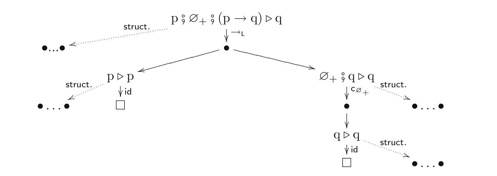
The •-nodes are suggestively dubbed or-nodes, their children are dubbed and-nodes. This nomenclature proposes the following inductive reading of provability within a space of reductions: a sequent is provable if and only if it is either vacuous (i.e., it is $\Box$) or all the children of at least one of its or-nodes are provable.
Let S be a sequent. A finite subtree R of a space of reductions $\rhoL(S)$ is an L-reduction of S iff the root of R is S and the immediate sub-trees of R are reductions $R_1, \ldots, R_n$ are precisely reductions of the sequents in $\{s_1, \ldots, s_n\} \in \rhoL(S)$. A reduction is successful iff all the leaves are $\Box$.
The sub-tree that is explicit in Example 3.2 is a reduction for $p \rsemi \emptyset_+ \rsemi (p \to q) \rhd q$ in that space. It is a successful reduction because the terminal nodes are all $\Box$.
A tree of sequents T is an L-proof of S if and only if T is a successful L-reduction of S.
Immediate by induction on the height of proofs and the definition of reduction tree—see, for example, previous work by the authors [15].
The idea of this paper is that reasoning about judgments (i.e., analyzing and determining why one obtains for a given sequent) may be formal characterized by exploring a space of reductions capturing the possible inferences that lead to the conclusion. For example, we mean by proof-theoretic reasoning the systematic analysis of the rules from a proof system to establish the conditions under which a sequent may be deemed provable in that system. In particular, we reason backward from the sequent through the space of reductions, concentrating on those reductions that are successful, if there are any. Taking the stance that this captures a common form of reasoning used in mathematics, we apply it to reasoning about validity.
The technology delivering this paper is that one can take the phrase model theory literally. This is the subject of Section 4. Essentially, one may study satisfaction in a frame as a theory of first-order classical logic by formalizing the implicit ambient logic in which mathematics is conducted as a meta-logic. Being classical, the meta-logic comes with its own wellunderstood and well-behaved proof theory, and one uses the construction of space of reductions with respect to the meta-calculus to characterize modeltheoretic reasoning. Reasoning proof-theoretically about the clauses of the semantics for BI (i.e., Figure 4) encoded within the meta-logic reveals that they actually have the same behaviour as the rules of sLBI. Thus proving soundness and completeness amounts to showing that the space of reductions for validity for any given sequent is, essentially, the same as the space of reductions for provability for the same sequent.
□4 Model Theory qua Classical Theory
In this section we capture BI-frames and satisfaction as a theory of a firstorder classical logic, called the meta-logic, in such a way that a validity judgment obtain iff there is a formal proof of a corresponding meta-sequent. The section is composed of three parts: in Section 4.1, we define the metalogic and the encoding of validity; in Section 4.2, we develop a sequent calculus, called the meta-calculus, for the meta-logic suitable to our needs; in Section 4.3, we demonstrate that reasoning about validity is captured by reduction in the meta-calculus.
4.1 The Meta-logic
The mathematics used to study logic happens itself within a logic, which may be called the ambient logic. In this section we formalize the ambient logic into a symbolic (meta-)logic that allows us to study model theory systematically. This move is quite natural as an early use of logic was to understand symbolically the logic in which mathematical reasoning takes places; for example, such uses of logics are used to study the natural numbers (i.e., by theories of arithmetic such as PA), set theory (e.g., by theories such as ZF(C)), etc. From this perspective, the present paper differs only in that the application is to study another logic—that is, BI. This is closely related to the relational calculi introduced by Negri [23] for modal logic. The meta-logic introduced in this section is designed for the model theory of BI. The guiding principle is to encode the definitions of the previous section symbolically as directly as possible.
The syntax is a two-sorted firstorder alphabet, the sorts are world and formulas. Let $\mathbb{V}_w$ be the set world-variables, and let $\mathbb{V}_f$ be the set of formulavariables, and fix world-constants e and $\pi$. The set of world-terms $\mathbb{T}_w$ is comprised of $\mathbb{V}_w$, e and $\pi$, and the set of formula-terms $\mathbb{T}_f$ is generated by using the connectives of BI as function symbols, $$\varphi ::= p \in \mathbb{P} \mid x_f \in \mathbb{V}_f \mid \top \mid \bot \mid \top^* \mid \varphi \land \psi \mid \varphi \lor \psi \mid \varphi \to \varphi \mid \varphi \ast \varphi \mid \varphi \wand \varphi$$ The set of meta-atoms $\mathbb{A}$ is comprised of $(x \Vdash \varphi)$, $R(x, y, z)$, $(x \preceq y)$, $(x = y)$ for $x, y, z \in \mathbb{V}_w \cup \{e, \pi\}$ and $\varphi \in \mathbb{T}_f$. The set of meta-formulas $\mathbb{M}$ is defined by the following grammar: $$\Phi ::= A \in \mathbb{A} \mid \Phi \mathbin{\&} \Phi \mid \Phi \parr \Phi \mid \Phi \Rightarrow \Phi \mid \forall\varphi\Phi \mid \forall w\Phi \mid \exists w\Phi \mid \exists\varphi\Phi \mid \Box$$ We are overloading a lot of notation, but in every case the symbol in the meta-logic is intended to denote the mathematical object for which we have the same notation; for example, the symbol $\Vdash$ is overloaded as both a relation symbol in the meta-logic and the satisfaction relation of BI. Henceforth, in the context of the meta-logic, we may write $\varphi$ to denote a formula-term. We write $(w \Vdash \Gamma)$ to abbreviate the meta atom $(w \Vdash \lfloor\Gamma\rfloor)$. The notation $\Phi \Leftrightarrow \Psi$ abbreviates $(\Phi \Rightarrow \Psi) \mathbin{\&} (\Psi \Rightarrow \Phi)$. For the sake of economy, we identify meta-formulas of the form $\Phi \Rightarrow \Psi$ with $\Phi \Leftarrow \Psi$. Throughout, the symbols $\Sigma$ and $\Pi$ are reserved for lists of meta-formulas; $\Sigma \sim \Sigma'$ denotes that $\Sigma$ and $\Sigma'$ are permutations of each other. We call meta-atoms of the form $(w \Vdash \varphi)$ assertions.
A meta-sequent is a pair $\Sigma \rhd \Pi$ in which $\Sigma$ and $\Pi$ are lists of meta-formulas. The empty pair, denoted $\Box$, is also a sequent. A meta-sequent is an unjudged structure; for example $p \rhd \bot$ is a metasequent. The consequence judgment for the meta-logic is first-order classical consequence.
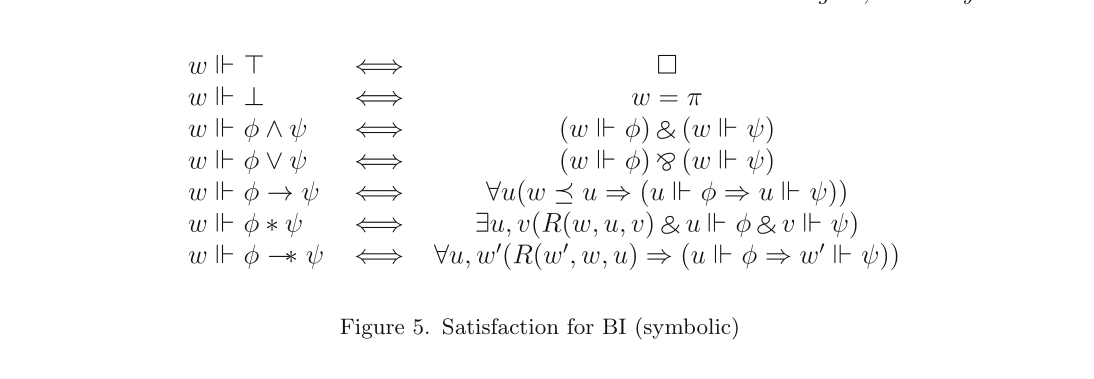
A meta-sequent $\Sigma \rhd \Pi$ is a meta—consequence—denoted $\Sigma \blacktriangleright \Pi$ — iff $\Sigma \rhd \Pi$ is a consequence of firstorder classical logic. We aim to develop a list of meta-formulas $\Omega$ such that $\Omega, (w \Vdash \Gamma) \blacktriangleright (w \Vdash \Delta)$ iff $\Gamma \vDash \Delta$. This is the task of the remainder of this section. The definitions of the previous section can be encoded in the meta-logic; that is, one may regard the model theory of BI qua a theory in the metalogic. There are two parts to capture: the sentences governing BI-frames $\Omega_{\mathfrak{M}}$ (Definition 2.18) and sentences governing satisfaction $\Omega_{\Vdash}$ (Definition 2.17). The sentences in $\Omega_{\mathfrak{M}}$ are the universal closure of the following, in which u, v, w, x, y, z are world-variables and $\varphi$ is a formula variable: $$\underbrace{R(x, x, e)}_{\text{unitality}} \qquad \underbrace{R(x, y, z) \Leftrightarrow R(x, z, y)}_{\text{commutativity}} \qquad \underbrace{w \preceq u \Rightarrow (w \Vdash \varphi \Rightarrow u \Vdash \varphi)}_{\text{persistence}}$$ $$\underbrace{R(x, w, y) \mathbin{\&} R(y, u, v) \Rightarrow \exists z(R(x, z, v) \mathbin{\&} R(z, w, u))}_{\text{associativity}} \qquad \underbrace{w = \pi \Rightarrow w \Vdash \varphi}_{\text{absurdity}}$$ The sentences in $\Omega_{\Vdash}$ are given by the universal closure of the metaformulas in Figure 5, which merits comparison with Figure 4, in which quantifiers are taken to be over each implicit conjunct separately in the bi-implications. There are two significant differences between Figs. 4 and 5: first, there is no clause for $(w \Vdash p)$, where $p \in \mathbb{P}$; second, there is no clause for $(w \Vdash \top^*)$. This is an effort to simplify computations about satisfaction in subsequent parts of the paper.
The elimination of a clause for atomic satisfaction follows from working with validity directly (i.e., without passing though truth-in-a-model) as interpretations are no longer required; that is, atomic satisfaction is captured by an atomic tautology, $\Omega, (w \Vdash p) \blacktriangleright (w \Vdash p)$. We justify the omission of an encoding for the $\top^*$-clause at end of this section. The concatenation of $\Omega_{\Vdash}$ and $\Omega_{\mathfrak{M}}$ is the desired theory $\Omega$. Indeed, $$\Omega, (w \Vdash \Gamma) \blacktriangleright (w \Vdash \varphi) \;\text{ iff }\; \Gamma \vDash \varphi$$ The significance of this is that all the familiar tools of classical logic become available, including sequent calculi for reasoning about when the above implication holds. The details of the proof-theoretic tools used for the metalogic in this paper is reserved for Section 4.2.
A basic validity sequent (BVS) is a meta-sequent $\Omega, (w \Vdash \Gamma) \rhd (w \Vdash \varphi)$.
A complex validity sequent (CVS) is a meta-sequent $\Omega, \bar{\Sigma} \rhd \bar{\Pi}$ in which $\bar{\Sigma}$ and $\bar{\Pi}$ are sets of assertions. To conclude this section, we explain why the $\top^*$-clause of satisfaction may be omitted in $\Omega$. Let $\Phi_{\top^*} := \forall x\big((x \Vdash \top^*) \Leftrightarrow (e \preceq x)\big)$, we claim $\Omega, (w \Vdash \Gamma) \blacktriangleright (w \Vdash \top^*)$ iff $\Omega, \Phi_{\top^*}, (w \Vdash \Gamma) \blacktriangleright (w \Vdash \top^*)$. This follows from the fact that $\Omega, \Phi_{\top^*}, (w \Vdash \Gamma) \blacktriangleright (w \Vdash \top^*)$ iff $\Gamma \vDash \top^*$, which is what we would expect for a model of BI, but then we already have $\Omega, (w \Vdash \Gamma) \blacktriangleright (w \Vdash \top^*)$. In short, the $\top^*$-clause can be removed from BI-frames without loss of generality when encoding in the meta-logic because the sequent calculus rule governing $\top^*$ requires that $\top^*$ is already part of the context—indeed, this is the same reason satisfaction of atoms could be eliminated. The other atomic rules, such as $\top$ and $\bot$ do not satisfy this condition, therefore their clauses are required.
4.2 Proof Theory for the Meta-logic
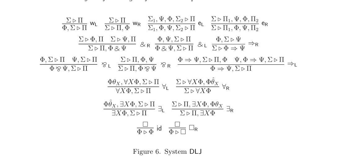
Having encoded the (putative) semantics of BI as a theory of the meta-logic, all of the tools of first-order classical logic become available. In particular, that a meta-sequent is a consequence of the meta-logic may be established by witnessing a proof for it in a proof system for first-order classical logic. In this section, we develop a sequent calculus for the meta-logic that is tractable for analyzing the semantics. The logic of BI is constructive. Consequently, one expects satisfaction to be constructive in the sense that, if $\Omega, (w \Vdash \Gamma) \blacktriangleright (w \Vdash \varphi)$ obtains, then there should be a constructive proof of it. Therefore, we may restrict to an intuitionistic sequent calculus for the meta-logic. This sequent calculus need only be sound and complete for BVSs that are valid in classical logic, we do not require it to be sound and complete for the whole logic. The following is based on Dummett’s [11] multiple-conclusioned system for first-order IL:
System DLJ is composed of the rules in Figure 6 in which $\theta_X$ denotes a substitution for X and $\hat{\theta}_X$ denotes a substitution for X by an eigenvariable. We elide rules for negation from Figure 6 as $\Omega$ is negation-free, so they will not be required at any point. We may use double-lines to suppress the use of multiple inference; for example, we may write $$\dfrac{\Phi, \Phi', \Phi'' \rhd \Pi}{(\Phi \mathbin{\&} \Phi') \mathbin{\&} \Phi'' \rhd \Pi}\,{\&}\mathrm{R}$$ to denote compactly the repeated use of ${\&}_L$ — that is, to express the following: $$\dfrac{\dfrac{\Phi, \Phi', \Phi'' \rhd \Pi}{\Phi \mathbin{\&} \Phi', \Phi'' \rhd \Pi}\,{\&}\mathrm{R}}{(\Phi \mathbin{\&} \Phi') \mathbin{\&} \Phi'' \rhd \Pi}\,{\&}\mathrm{R}$$ The encoding of Section 4.1 is in a classical meta-logic and thus, despite the above intuition, we have no guarantee that DLJ is adequate for proving BVSs. To this end, it suffices to show that the following rules are admissible for DLJ-proofs of BVSs as including them recovers a meta-sequent calculus for classical logic: $$\dfrac{\Sigma \rhd \Pi, \Phi}{\Sigma \rhd \Pi, \forall x\Phi}\,{\forall^{K}_{R}} \qquad \dfrac{\Phi, \Sigma \rhd \Pi, \Psi}{\Sigma \rhd \Pi, \Phi \Rightarrow \Psi}\,{\Rightarrow^{K}_{R}} \qquad \dfrac{\Sigma \rhd \Pi, \Phi, \Phi}{\Sigma \rhd \Pi, \Phi}\,{c_R} \qquad \dfrac{\Phi, \Phi, \Sigma \rhd \Pi}{\Phi, \Sigma \rhd \Pi}\,{c_L}$$ Two rules are immediate:
The $c_R$-rule and $c_L$-rule are admissible in DLJ.
Follows from the idempotency of intuitionistic disjunction and intuitionistic conjunction. That is, since $\Phi \Leftrightarrow \Phi \parr \Phi$ is valid in intuitionistic logic, $\Sigma \vdash_{DLJ} \Pi, \Phi$ obtains iff $\Sigma \vdash_{DLJ} \Pi, \Phi \parr \Phi$ obtains; similarly, since $\Phi \Leftrightarrow \Phi \mathbin{\&} \Phi$ is valid in intuitionistic logic, $\Phi, \Sigma \vdash_{DLJ} \Pi$ obtains iff $\Phi \mathbin{\&} \Phi, \Sigma \vdash_{DLJ} \Pi$ obtains. The result follows from application of the application of ${\&}_R$ and ${\&}_L$. The remaining two rules (i.e., $\forall^{K}_{R}$ and $\Rightarrow^{K}_{R}$) are generalized versions of $\forall_R$ and $\Rightarrow_R$, respectively. Define $DLJ^K := DLJ \cup \{\forall^{K}_{R}, \Rightarrow^{K}_{R}, c_R, c_L\}$. The relationship between DLJ and DLJK is the same as the relationship between Dummett’s [11] (multiple-conclusioned) sequent calculus for IPL and Gentzen’s [31] LK—that is, that certain rules in the former system are guarded by a single-conlusioned condition that, if relaxed (or, generalized—see previous work by the authors [15]) to be multiple-conclusioned, recovers the latter system. Why can this guard be removed for proofs of BVSs without effecting completeness of the calculus? A sufficient guard is already captured. We shall return to this idea once a certain definitions and technical results have been given that will facilitate the discussion.
Rather than consider proofs (or reductions) for the meta-logic in general, we restrict attention to CVSs and, eventually, BVSs. In particular, we consider reductions that use a meta-formula in $\Omega.$ Such steps are called resolutions.
□A resolution is a derivation that instantiates a clause from $\Omega$ by applying the $\forall_L$-rule, then applies the $\Rightarrow_L$-rule on the resulting sub-formula, and then removes the sub-formula, $$\dfrac{\dfrac{\dfrac{\Omega, \Sigma \rhd \Pi, \Phi}{\Omega, \Phi \Rightarrow \Psi, \Sigma \rhd \Pi, \Phi}\,w_L \qquad \dfrac{\Omega, \Psi, \Sigma \rhd \Pi}{\Omega, \Phi \Rightarrow \Psi, \Psi, \Sigma \rhd \Pi}\,w_L}{\Omega, \Phi \Rightarrow \Psi, \Sigma \rhd \Pi}\,{\Rightarrow_L}}{\Omega, \Sigma \rhd \Pi}\,\forall_L$$ A resolution is closed if the head of the clause matches with an assertion already present in the meta-sequent, and one removes (by using $w_L$ or $w_R$) the head in the non-axiom premiss, $$\dfrac{\dfrac{\Box}{\Omega, \Phi, \Sigma \rhd \Pi, \Phi} \qquad \Omega, \Psi, \Phi, \Sigma \rhd \Pi}{\Omega, \Phi, \Sigma \rhd \Pi}\,w_L \qquad\qquad \dfrac{\Omega, \Sigma \rhd \Pi, \Phi \qquad \dfrac{\Box}{\Omega, \Psi, \Sigma \rhd \Pi, \Psi}}{\Omega, \Sigma \rhd \Pi, \Psi}\,w_R$$ It is without loss of generality that we reduce with $\Rightarrow_L$ immediately after reducing with $\forall_L$ as the quantifier rule is invertible.
Intuitively, a closed resolution is a resolution in which the consequent of the implication replaces the formula that matches the antecedent. A resolution is open iff it is not closed. When a resolution is closed, we may denote the reduction by the premiss that is not a tautology, labeling it by the name of the justifying metaformula. That is, let f be name of some formula in $\Omega$ that instantiates to $\Phi \Rightarrow \Psi$, then closed resolutions using f are as follows: $$\dfrac{\Omega, \Psi, \Sigma \rhd \Pi}{\Omega, \Phi, \Sigma \rhd \Pi}\,f_L \qquad\qquad \dfrac{\Omega, \Sigma \rhd \Pi, \Phi}{\Omega, \Sigma \rhd \Pi, \Psi}\,f_R$$ When no confusion arises, we may suppress the left or right subscript on these inference. Denoted in this way, resolutions may be thought of as rules (or, more precisely, as reduction operators). This allows us to emphazise the steps that make use of the theory $\Omega$ while de-emphasizing the meta-logical ones.
Reasoning that $\Gamma \vDash \varphi \land \psi$ arrives from $\Gamma \vDash \varphi$ and $\Gamma \vDash \psi$ is represented in the meta-logic by a closed resolution using the $\land$-clause, $$\dfrac{\dfrac{\dfrac{\Omega, (w \Vdash \Gamma) \rhd (w \Vdash \varphi) \qquad \Omega, (w \Vdash \Gamma) \rhd (w \Vdash \psi)}{\Omega, (w \Vdash \Gamma) \rhd (w \Vdash \varphi) \mathbin{\&} (w \Vdash \psi)}}{\Omega, (w \Vdash \Gamma) \rhd (w \Vdash \varphi) \mathbin{\&} (w \Vdash \psi), (w \Vdash \varphi \land \psi)}\,w_R \qquad \dfrac{\Box}{\;}\,\text{id}}{\Omega, (w \Vdash \Gamma) \rhd (w \Vdash \varphi \land \psi)}$$ We suppress the conclusion of the id-rule for readability, it has the metaformula $(w \Vdash \varphi\land\psi)$ in both the context and the extract. Using the compact notation for closed-resolutions, the same derivation may be denoted as follows: $$\dfrac{\dfrac{\Omega, (w \Vdash \Gamma) \rhd (w \Vdash \varphi) \qquad \Omega, (w \Vdash \Gamma) \rhd (w \Vdash \psi)}{\Omega, (w \Vdash \Gamma) \rhd (w \Vdash \varphi) \mathbin{\&} (w \Vdash \psi)}\,{\&}\mathrm{R}}{\Omega, (w \Vdash \Gamma) \rhd (w \Vdash \varphi \land \psi)}\,{\land}\text{-clause}$$ Since the theory $\Omega$ is conserved in DLJ-reductions, henceforth we may suppress it without further comment.
It is reasoning by resolution that captures what it means to use a clause of satisfaction, hence the sequent calculus for the meta-logic ought to have resolutions as the primary operational step during reduction. The fact that resolution is how semantic reasoning is conducted is not surprising; after all, that a theory composed of clauses may be used to define a predicate is the idea underpinning Logic Programming (LP)—see Kowalski [18,19]. Resolutions can be used not only to perform computation about the satisfaction relation, but to break up the structure of bunches such that they may be read in the form of a classical context. We may think of this as unpacking the bunch. Of course, it is essential that no information is lost in this process.
An unpacking of a meta-atom $(w \Vdash \Gamma)$ in a meta-sequent $\Omega, \Sigma, (w \Vdash \Gamma) \rhd \Pi$ is a sequence of closed resolutions using $\land$- and $\ast$-clauses in the context with $\exists_L$ and ${\&}_L$ applied eagerly. A packing is the reverse of an unpacking.
The following computation constitutes an unpacking of the meta-formula $(w \Vdash \Gamma \rcomma (\Delta \rsemi \Delta'))$ in the meta-sequent $(w \Vdash \Gamma \rcomma (\Delta \rsemi \Delta')), (u \Vdash \Gamma') \rhd (w \Vdash \varphi), (u \Vdash \psi)$: $$\dfrac{\dfrac{\dfrac{\dfrac{R(w, x, y), (x \Vdash \Gamma), (y \Vdash \Delta) \mathbin{\&} (y \Vdash \Delta'), (u \Vdash \Gamma') \rhd (w \Vdash \varphi), (u \Vdash \psi)}{R(w, x, y), (x \Vdash \Gamma), (y \Vdash \Delta \rsemi \Delta'), (u \Vdash \Gamma') \rhd (w \Vdash \varphi), (u \Vdash \psi)}\,{\land}\text{-clause}}{R(w, x, y) \mathbin{\&} (x \Vdash \Gamma) \mathbin{\&} (y \Vdash \Delta \rsemi \Delta'), (u \Vdash \Gamma') \rhd (w \Vdash \varphi), (u \Vdash \psi)}\,{\&}_L}{\exists x, y\big(R(w, x, y) \mathbin{\&} x \Vdash \Gamma \mathbin{\&} y \Vdash \Delta \rsemi \Delta'\big), (u \Vdash \Gamma') \rhd (w \Vdash \varphi), (u \Vdash \psi)}\,\exists_L}{(w \Vdash \Gamma \rcomma (\Delta \rsemi \Delta')), (u \Vdash \Gamma') \rhd (w \Vdash \varphi), (u \Vdash \psi)}\,{\ast}\text{-clause}$$ The notation $\Sigma_{w,\Gamma}$ denotes a theory that arises from an unpacking of $(w \Vdash \Gamma)$. Unpackings do not have to be total—that is, one can have $w \Vdash \Gamma(\varphi)$ unpack to a theory $\Sigma_{w,\Gamma(\varphi)}$ containing a meta-formula $x \Vdash \varphi$. In this case, the theory may be denoted $\Sigma_{w,\Gamma(\varphi),x\Vdash\varphi}$. It is partial in the sense that the unpacking does not continue on the assertion $w \Vdash \varphi$,
Both packing and unpackings are invertible.
The result follows from the invertibility of ${\&}_L$ and $\exists_L$, as witnessed by the following computations in which we use dashed lines to represent the inverse of a rule: $$\dfrac{\dfrac{\dfrac{\dfrac{\Sigma, (w \Vdash \varphi \land \psi) \rhd \Pi}{\Sigma, (w \Vdash \varphi) \mathbin{\&} (w \Vdash \psi) \rhd \Pi}\,{\land}\text{-clause}}{\Sigma, (w \Vdash \varphi), (w \Vdash \psi) \rhd \Pi}\,{\&}_L^{-1}}{\Sigma, (w \Vdash \varphi) \mathbin{\&} (w \Vdash \psi) \rhd \Pi}\,{\&}_L}{\Sigma, (w \Vdash \varphi \land \psi) \rhd \Pi}\,{\land}\text{-clause}$$ $$\dfrac{\dfrac{\dfrac{\dfrac{\dfrac{\dfrac{\Sigma, (w \Vdash \varphi \ast \psi) \rhd \Pi}{\Sigma, \exists u, v\big(R(w, u, v) \mathbin{\&} (u \Vdash \varphi) \mathbin{\&} (v \Vdash \psi)\big) \rhd \Pi}\,{\ast}\text{-clause}}{\Sigma, R(w, u, v) \mathbin{\&} (u \Vdash \varphi) \mathbin{\&} (v \Vdash \psi) \rhd \Pi}\,\exists_L^{-1}}{\Sigma, R(w, u, v), (u \Vdash \varphi), (v \Vdash \psi) \rhd \Pi}\,{\&}_L^{-1}}{\Sigma, R(w, u, v) \mathbin{\&} (u \Vdash \varphi) \mathbin{\&} (v \Vdash \psi) \rhd \Pi}\,{\&}_L}{\Sigma, \exists u, v\big(R(w, u, v) \mathbin{\&} (u \Vdash \varphi) \mathbin{\&} (v \Vdash \psi)\big) \rhd \Pi}\,\exists_L}{\Sigma, (w \Vdash \varphi \ast \psi) \rhd \Pi}\,{\ast}\text{-clause}$$ We may now return to the question of the adequacy of DLJ for BVSs despite being intuitionistic. Heuristically, one expects DLJ to be adequate because the guard distinguishing $\Rightarrow_R$ and $\forall_R$ from $\Rightarrow^{K}_{R}$ and $\forall^{K}_{R}$ is captured by the change of world when encountering an implication formula in the extract of a CVS. This idea is witnessed in the following example:
□To see how the change of world acts as a sufficient guard for BI-validity to be constructive, we may see how DLJK avoids the law of the excluded middle (i.e., why $(w \Vdash \emptyset_\times) \rhd (w \Vdash \varphi \lor (\varphi \to \bot))$ from holding in BI: $$\dfrac{\dfrac{\dfrac{\dfrac{\dfrac{\dfrac{\dfrac{(w \Vdash \emptyset_\times), (u \Vdash \emptyset_\times \rsemi \varphi) \rhd (w \Vdash \varphi), (u \Vdash \bot)}{(w \Vdash \emptyset_\times), (u \Vdash \emptyset_\times), (u \Vdash \varphi) \rhd (w \Vdash \varphi), (u \Vdash \bot)}\,{\land}\text{-clause}}{(w \Vdash \emptyset_\times), u \preceq w, (u \Vdash \varphi) \rhd (w \Vdash \varphi), (u \Vdash \bot)}\,\text{pers.}}{(w \Vdash \emptyset_\times) \rhd (w \Vdash \varphi), (w \preceq u \Rightarrow (u \Vdash \varphi \Rightarrow u \Vdash \bot))}\,{\Rightarrow^{K}_{R}}}{(w \Vdash \emptyset_\times) \rhd (w \Vdash \varphi), \forall u(w \preceq u \Rightarrow (u \Vdash \varphi \Rightarrow u \Vdash \bot))}\,{\forall^{K}_{R}}}{(w \Vdash \emptyset_\times) \rhd (w \Vdash \varphi), (w \Vdash (\varphi \to \bot))}\,{\to}\text{-clause}}{(w \Vdash \emptyset_\times) \rhd (w \Vdash \varphi) \parr (w \Vdash (\varphi \to \bot))}\,{\parr}\mathrm{R}}{(w \Vdash \emptyset_\times) \rhd (w \Vdash \varphi \lor (\varphi \to \bot))}\,{\lor}\text{-clause}$$
Moving to u and using persistence means that one has all the contextual information about w available (i.e., that $w \Vdash \Gamma$ is in the context enables $u \Vdash \Gamma$ to be assumed); but since $u \Vdash \varphi$ in the context and $w \Vdash \varphi$ in the extract are different atoms since u and w are distinct, one has not reached an axiom. In short despite working in a classical system (i.e., DLKK), suppressing an additional computational step, the above calculation witnesses that $\emptyset_\times \vDash$ $\varphi \lor \varphi \to \bot$ if $\emptyset_\times \vDash \varphi$ or $\varphi \vDash \bot$, which is what one would expect of entailment for a constructive logic such as BI. The way the change-of-world guard works is that the CVS to which one reduces when resolving an implications assertion contains two independent claims about validity, as witnessed in Example 4.13, which may be separated out.
Sets of meta-formulas $\Sigma$ and $\Sigma'$ are world-independent if no free world-variable appearing in one appears in the other.
Let $\Sigma, \Sigma', \Pi, \Pi'$ be sets of propositional meta-formulas such that $\Sigma, \Pi$ and $\Sigma', \Pi'$ are world-independent: $$\Omega, \Sigma, \Sigma' \rhd \Pi, \Pi' \;\text{ iff }\; \Omega, \Sigma \rhd \Pi \;\text{ or }\; \Omega, \Sigma' \rhd \Pi'$$ Recall that $\Omega, \Sigma, \Sigma' \rhd \Pi, \Pi'$ obtains iff there there is a DLJK-proof of $\Omega, \Sigma, \Sigma' \rhd \Pi, \Pi'$. We proceed by by induction on DLJK-proofs. Note, the proof is sensitive to she shape of formulas in $\Omega$; for example, the induction step would fail if we had the linearity axiom $\forall x,y\,(x \preceq y \parr y \preceq x)$.
The if direction follows immediately by wL and wR. For the only if direction, assume $\Omega, \Sigma, \Sigma' \rhd \Pi, \Pi'$ and let D be a DLJK-proof of it. We proceed by induction the number of resolutions in D.
Base Case. If D contains no resolutions, then $\Omega, \Sigma, \Sigma' \rhd \Pi, \Pi'$ is proved by id together with the rules for the meta-connectives. But then there are proofs for $\Omega, \Sigma \rhd \Pi$ or $\Omega, \Sigma' \rhd \Pi'$ since the rules for the connectives cannot affect what world- or formula-variables.
Induction Step. Recall, without loss of generality, in DLJK, the $\forall_L$-rule is always followed by $\Rightarrow^{K}_{L}$. If a resolution of $\Omega, \Sigma, \Sigma' \rhd \Pi, \Pi'$ yields a metasequent of the form $\Omega, \Sigma \rhd \Pi$ or $\Omega, \Sigma' \rhd \Pi'$, then the result follows from the induction hypothesis. We show that this is the case.
The only non-obvious case is in the case of a closed resolution using the $\to$-clause or $\wand$-clause in the extract because they have universal quantifiers that would allow one to produce a meta-atom in the extract that contains both a world from $\Sigma, \Pi$ and $\Sigma', \Pi'$ simultaneously, thereby breaking worldindependence. We show the $\to$-case, the other being similar.
Let $\Sigma = \Sigma'', w \Vdash \varphi \to \psi$ and suppose u is a world variable appearing in $\Sigma', \Pi'$, then we have the following computation: $$\dfrac{\dfrac{\dfrac{\Omega, \Sigma'', \Sigma' \rhd \Pi, \Pi', w \preceq u \quad \Omega, \Sigma'', \Sigma' \rhd \Pi, \Pi', (u \Vdash \varphi) \quad \Omega, \Sigma'', \Sigma', (u \Vdash \psi) \rhd \Pi, \Pi'}{\Omega, \Sigma'', (w \preceq u \Rightarrow (u \Vdash \varphi \Rightarrow u \Vdash \psi)), \Sigma' \rhd \Pi, \Pi'}\,{\Rightarrow^{K}_{L}}}{\Omega, \Sigma'', \forall x(w \preceq x \Rightarrow (x \Vdash \varphi \Rightarrow x \Vdash \psi)), \Sigma' \rhd \Pi, \Pi'}\,\forall_L}{\Omega, \Sigma'', (w \Vdash \varphi \to \psi), \Sigma' \rhd \Pi, \Pi'}\,{\to}\text{-clause}$$ The meta-atom $(w \preceq u)$ may be removed from the leftmost premiss because the only way for the meta-atom to be used in the remainder of the proof is if $w \preceq u$ appears in the context, but this is impossible. Hence, without loss of generality, D applies wR to the branch, yielding $\Sigma'', \Sigma' \rhd \Pi, \Pi'$, as required.
To prove that DLJ is adequate for proofs of CVSs it only remains to argue that the change-of-world guard is implemented whenever it is required, and that it indeed results in a world-independent situation.
□The $\forall K$ R and $\RightarrowK$ R rules are admissible for DLJ-proofs of CVSs:
By case analysis on $\Omega$, the only place on may require $\forall^{K}_{R}$ or $\Rightarrow^{K}_{R}$ over $\forall_R$ or $\Rightarrow_R$ is when resolving an implicational assertion (i.e., using the $\to$-clause or the $\wand$-clause).
This is because they are the only clauses whose bodies contain implications; notably, the clause for $\ast$ does not contain a meta-implication, and this is so that it behaves like a conjunction, which delivers the packing and unpacking above, as well as completeness.
In the case of $\to$-clause, without loss of generality, the resolution may be taken to be required for the proof such that persistence is applied eventually to the meta-atom $(w \preceq u)$ producing by the resolution. By permuting resolutions, we may assume that it is used immediately. By Lemma 4.12, these reductions are followed by a packing: $$\dfrac{\dfrac{\dfrac{\dfrac{\bar{\Sigma}, (w \Vdash \Gamma), (u \Vdash \Gamma \rsemi \varphi) \rhd \bar{\Pi}, (u \Vdash \psi)}{\bar{\Sigma}, (w \Vdash \Gamma), (u \Vdash \Gamma), (u \Vdash \varphi) \rhd \bar{\Pi}, (u \Vdash \psi)}\,{\land}\text{-clause}}{\bar{\Sigma}, (w \Vdash \Gamma), w \preceq u, (u \Vdash \varphi) \rhd \bar{\Pi}, (u \Vdash \psi)}\,\text{pers.}}{\bar{\Sigma}, (w \Vdash \Gamma) \rhd \bar{\Pi}, (w \preceq u \Rightarrow (u \Vdash \varphi \Rightarrow u \Vdash \psi))}\,{\Rightarrow^{K}_{R}}}{\bar{\Sigma}, (w \Vdash \Gamma) \rhd \bar{\Pi}, \forall u(w \preceq u \Rightarrow (u \Vdash \varphi \Rightarrow u \Vdash \psi))}\,{\forall^{K}_{R}}$$ Arguing similarly, in the case of the $\wand$-clause, one has the following derivation: $$\dfrac{\dfrac{\dfrac{\bar{\Sigma}, (w \Vdash \Gamma), (w' \Vdash \Gamma \rcomma \varphi) \rhd \bar{\Pi}, (w' \Vdash \psi)}{\bar{\Sigma}, (w \Vdash \Gamma), R(w', w, u), u \Vdash \varphi \rhd \bar{\Pi}, (w' \Vdash \psi)}\,{\ast}\text{-clause}}{\bar{\Sigma}, (w \Vdash \Gamma) \rhd \bar{\Pi}, (R(w', w, u) \Rightarrow (u \Vdash \varphi \Rightarrow w' \Vdash \psi))}\,{\Rightarrow^{K}_{R}}}{\bar{\Sigma}, (w \Vdash \Gamma) \rhd \bar{\Pi}, \forall w', u(R(w', w, u) \Rightarrow (u \Vdash \varphi \Rightarrow w' \Vdash \psi))}\,{\forall^{K}_{R}}$$ In either case, by the eigenvariable condition on universal instantiations, the premiss is a meta-sequent of the form $\Omega, \Sigma, \Sigma' \rhd \Pi, \Pi'$ in which $\Sigma, \Pi$ and $\Sigma', \Pi'$ are world-independent. Hence, by Lemma 4.15, one yields premisses that one may have reached using the single-conclusioned variants of the rules; whence, the multiple-conclusioned variants are admissible. The adequacy of DLJ follows as a corollary from the preceeding work.
□A CVS holds iff it admits a DLJ-proof.
Immediate by Lemmas 4.16 and 4.7. In the remainder of this section, we eliminate a particular behaviours from DLJ in order to simplify the analysis of the space of reductions for a given CVS: the possibility of introducing world-variables that are irrelevant. When reducing a CVS, it is possible to instantiate a meta-formula in $\Omega$ with a world not present in the meta-sequent, but such a world-variable represents an arbitrary world alien to information about models available in the sequent and therefore, intuitively, it cannot be a required part of the reasoning used to establish or refute the CVS.
□The following derivation is a reduction of a BVS that begins with a resolution introducing a world alien to the original meta-sequent: $$\dfrac{\dfrac{\Omega, (w \Vdash p \land q) \rhd (u \Vdash \top) \qquad \Omega, (w \Vdash p \land q) \rhd (w \Vdash p \lor q)}{\Omega, (u \Vdash \top) \Rightarrow \Box, (w \Vdash p \land q) \rhd (w \Vdash p \lor q)}\,{\Rightarrow_L}}{\Omega, (w \Vdash p \land q) \rhd (w \Vdash p \lor q)}\,\forall_L$$ We eliminate computation such as in Example 4.18 so that after resolutions way may always interpret meta-sequents as BI-sequents (see Section 4.3, below).
A DLJ-proof of a CVS is said to be world-conservative if in any instance of $\forall L$ or $\exists R,$ every world-variable occurring in the premiss occurs in the conclusion.
A CVS holds iff it admits a world-conservative DLJ-proof.
Since $\forall L$ has no pre-conditions, the result follows from Lemma 4.17 by renaming variables. That is, suppose a DLJ-proof contains the following inference that is not world-conservative (i.e., $\theta_u : u \mapsto x$ and x does not appear in $\Sigma$ or $\Pi$): $$\dfrac{\Omega, \Sigma, \Psi\theta_u \rhd \Pi}{\Omega, \Sigma, \forall u\Psi \rhd \Pi}$$ The proof can be made world-conservative by replacing all hereditary occurrences of x in the proof by a world-variable y that does appear in either $\Sigma$ or $\Pi$—for example, the above inference becomes the following, where $\theta'_u : u \mapsto y$: $$\dfrac{\Omega, \Sigma, \Psi\theta'_u \rhd \Pi}{\Omega, \Sigma, \forall u\Psi \rhd \Pi}$$ This substitution is then propagated up through the reduction.
Kreisel [20] has shown that there is no constructive proof of completeness for IPL with respect to its frame semantics. In this paper, the actual proof of completeness (i.e., Corollary 5.3) is certainly not constructive just because DLJ is constructive. Since the theory $\Omega$ is conserved in DLJ-reductions of BVSs, henceforth we may suppress it without further comment.
□4.3 Reasoning About BI-Validity
In this section, we give a meta-sequent calculus VBI, which is a restriction of DLJ that we use to characterize reasoning about validity. In particular, it is one in which closed resolutions are enforced precisely where we desire them. In the meta-logic, we address validity, bypassing truth-at-a-world, because the world-variables in meta-sequents do not stand for particular worlds, but rather are generic representatives of worlds. As such, we may call them eigenworlds.
Consider a meta-sequent $(w \Vdash r) \rhd (w \Vdash p \ast q)$, in which p, q, and r $\in \mathbb{P}$, to which we wish to apply the $\ast$-clause, $$\forall\varphi\forall\psi\forall x\big(\exists y\exists z(R(x, y, z) \mathbin{\&} y \Vdash \varphi \mathbin{\&} z \Vdash \psi) \Rightarrow x \Vdash \varphi \ast \psi\big)$$ Resolving with this clause produces the following meta-sequent: $$(w \Vdash r) \rhd \exists y, z\big(R(w, y, z) \mathbin{\&} (y \Vdash p) \mathbin{\&} (z \Vdash q)\big)$$ In the absence of any specific worlds, one introduces eigenworlds u and v to eliminate the existential quantifiers for y and z, respectively, yielding the following: $$(w \Vdash r) \rhd \big(R(w, u, v) \mathbin{\&} (u \Vdash p) \mathbin{\&} (v \Vdash q)\big)$$ This reasoning can take place at any world in any model; that is, suppose one were given an actual model M, then the above shows that if it holds for actual worlds a, b, c in M that R(c, a, b), $a \Vdash p$, and $b \Vdash q$ obtain, then necessarily $c \Vdash p \ast q$ also obtains. Our aim is to restrict to a meta-seqeunt calculus in which the possible ways in which one may reason about a BVS can be analyzed. To this end, we introduce a calculus for validity:
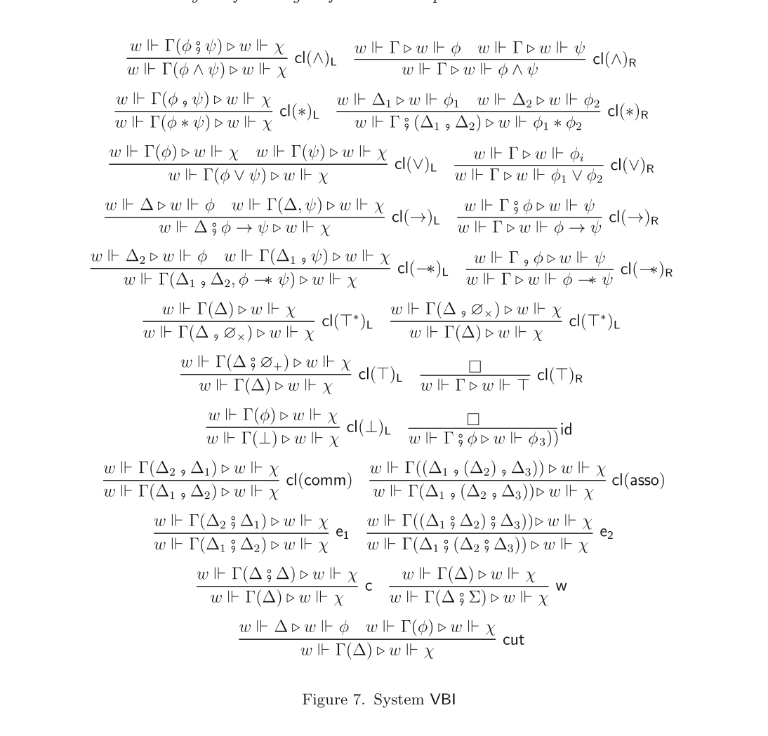
System VBI is composed of the rules in Figure 7 in which the theory $\Omega$ has been suppressed in the context and cl(asso) is invertible.
A BVS is valid iff it admits a VBI-proof.
The soundness of VBI is immediate by observing that each rule follows as the application of a meta-formula in $\Omega;$ for example, the admissibility of $cl(\land)R$ is witnessed in this way in Example 4.9. It remains to argue for the completeness of VBI.
By Lemma 4.20, a BVS is a consequence of the meta-logic iff it admits a world-conservative DLJ-proof. But since DLJ is an intuitionistic calculus, we have the same result for the single-conlusioned variant GLJ (i.e., the rules of DLJ with only one meta-formula in the extract and L forcing one to choose one disjunct). We proceed by case analysis on the possible reductions for the BVS in GLJ and show that they correspond to reductions in VBI. We may express that there is a reduction taking C to $P_1$, ..., Pn as follows: $P_1$ ... Pn C ⇑ In particular, if the reduction continues by taking Pi $Q_1$, ..., Qm the effect may be expressed as follows: $P_1$ ... Pi−1 $Q_1$ ... Qn Pi ...
Pn C ⇑ Without loss of generality, each reduction begins with an unpacking of the BVS. We may write $\Pi_{w,\Gamma(\Delta),x}, x \Vdash \Delta$ to denote a theory $\Sigma_{w,\Gamma(\Delta),x\Vdash\Delta}$. Moreover, without loss of generality, in the case of closed resolution, we assume that the resulting sub-formulas are immediately decomposed (i.e., are principal in the next reduction), as otherwise the resolution could have been postponed until this is the case.
By Lemma 4.12, we apply packing eagerly; that is, we apply it whenever it results in a sequent different from the original.
Of course, there are more
than one possible ways to pack a meta-sequent, but this is no concern as the possible choices simply correspond to $e_2$ $\in$ VBI. An example is offered by the following: $$\dfrac{\dfrac{(w \Vdash \Gamma((\Delta_1 \rsemi \Delta_2) \rsemi \Delta_3)) \rhd (w \Vdash \chi)}{\Pi_{w,\Gamma(\Delta_1\rsemi(\Delta_2\rsemi\Delta_3)),x}, (x \Vdash \Delta_1), (x \Vdash \Delta_2), (x \Vdash \Delta_3) \rhd (w \Vdash \chi)}\,\Uparrow}{(w \Vdash \Gamma(\Delta_1 \rsemi (\Delta_2 \rsemi \Delta_3))) \rhd (w \Vdash \chi)}\,\Uparrow$$ The reductions of BVSs GLJ begin with one of the following: an axiom, an open resolutions, a clause on an assertion in the extract, a clause on an assertion in the context, a frame law, or a structural rule. We structure the case-analysis into these groups for readability.
1. Axiom. System GLJ contains two axioms: id and $\Box$. Only one of them is applicable to the unpacking of a BVS — namely, id. If the reduction used id, then the unpacking of the BVS was of the form $\Sigma_{w,\Gamma}, (w \Vdash \varphi) \rhd (w \Vdash \varphi)$. This is only possible if the original BVS was of the form $(w \Vdash (\Gamma \rsemi \varphi)) \rhd (w \Vdash \varphi)$.
These reductions are captured by VBI as an instance of its version of id.
2. Open Resolutions. Recall, an open resolution is a resolution that is not closed — that is, one in which neither the antecedent nor the consequent of an instantiation of a meta-formula in $\Omega$ matches with any meta-formula in the meta-sequent. We consider the generic meta-sequent $(w \Vdash \Gamma(\Delta)) \rhd (w \Vdash \varphi)$, which is unpacked to $\Sigma_{w,\Gamma(\Delta),(x \Vdash \Delta)} \rhd (w \Vdash \varphi)$. A generic open resolution is as follows: $$\dfrac{\Sigma_{w,\Gamma(\Delta),(x \Vdash \Delta)} \rhd \Phi \qquad \Sigma_{w,\Gamma(\Delta),(x \Vdash \Delta)}, \Psi \rhd (w \Vdash \varphi)}{\Sigma_{w,\Gamma(\Delta),(x \Vdash \Delta)} \rhd (w \Vdash \varphi)}\,\Uparrow$$ By world-conservativity and by case-analysis on $\Omega$, it must be that, for some $\chi$, either $\Phi = (x \Vdash \chi)$ or $\Psi = (x \Vdash \chi)$. By the invertibility of the resolutions, we may continue with a closed-resolution to yield the following: $$\dfrac{\Sigma_{w,\Gamma(\Delta),(x \Vdash \Delta)} \rhd (x \Vdash \chi) \qquad \Sigma_{w,\Gamma(\Delta),(x \Vdash \Delta)}, (x \Vdash \chi) \rhd (w \Vdash \varphi)}{\Sigma_{w,\Gamma(\Delta),(x \Vdash \Delta)} \rhd (w \Vdash \varphi)}\,\Uparrow$$ By Lemma 4.15 and by Lemma 4.12, each branch is then weakened and packed. In total, the reduction from the original BVS is as follows: $$\dfrac{(x \Vdash \Delta) \rhd (x \Vdash \chi) \qquad (w \Vdash \Gamma(\Delta \rsemi \chi)) \rhd (w \Vdash \varphi)}{(w \Vdash \Gamma(\Delta)) \rhd (w \Vdash \varphi)}\,\Uparrow$$ Such reductions are captured by VBI as an instance of c followed by cut.
3. Extract-closed Resolutions. An extract-closed resolution is a closed resolution on a meta-formula in the extract. Without loss of generality, the unpacking at the beginning of each reduction is trivial when it is not required for the reduction to take place.
$\land$− Reductions beginning with the $\land$-clause are as follows: $$\dfrac{\dfrac{(w \Vdash \Gamma) \rhd (w \Vdash \varphi) \qquad (w \Vdash \Gamma) \rhd (w \Vdash \psi)}{(w \Vdash \Gamma) \rhd (w \Vdash \varphi) \mathbin{\&} (w \Vdash \psi)}\,{\&}\mathrm{R}}{(w \Vdash \Gamma) \rhd (w \Vdash \varphi \land \psi)}\,\Uparrow$$ These reductions are captured by VBI as $cl(\land)_R$. $\lor$− Reductions beginning with the $\lor$-clause are as follows: $$\dfrac{\dfrac{(w \Vdash \Gamma) \rhd (w \Vdash \varphi_i)}{(w \Vdash \Gamma) \rhd (w \Vdash \varphi_1) \parr (w \Vdash \varphi_2)}\,{\parr}\mathrm{R}}{(w \Vdash \Gamma) \rhd (w \Vdash \varphi \lor \psi)}\,\Uparrow$$ These reductions are captured by VBI as $cl(\lor)_R$. $\to$− Reductions beginning with the $\to$-clause are as follows: $$\dfrac{(w \Vdash \Gamma) \rhd (w \preceq u) \Rightarrow \big((u \Vdash \varphi) \Rightarrow (u \Vdash \psi)\big)}{(w \Vdash \Gamma) \rhd (w \Vdash \varphi \to \psi)}\,\Uparrow$$ By the invertibility of $\Rightarrow_R$, this is continued to yield the following: $$\dfrac{(w \Vdash \Gamma), (w \preceq u), (u \Vdash \varphi) \rhd (u \Vdash \psi)}{(w \Vdash \Gamma) \rhd (w \Vdash \varphi \to \psi)}\,\Uparrow$$ Without loss of generality, this reduction is continued by persistence. This follows by Lemma 4.15 as, if not, then $(w \Vdash \Gamma)$ and $(w \preceq u)$ may be removed without loss of completeness, but this removal can still happen after persistence. Moreover, by Lemma 4.12, the reduction is thence continued by a packing. In total, the reduction is as follows: $$\dfrac{(w \Vdash \Gamma \rsemi \varphi) \rhd (u \Vdash \psi)}{(w \Vdash \Gamma) \rhd (w \Vdash \varphi \to \psi)}\,\Uparrow$$ These reductions are captured by VBI as $cl(\to)_R$.
$\top$− Reductions beginning with the $\top$-clause are as follows: $$\dfrac{(w \Vdash \Gamma) \rhd \Box}{(w \Vdash \Gamma) \rhd (w \Vdash \top)}\,\Uparrow$$ Without loss of generality, the reduction ends by application of the $\Box_R$-axiom. These reductions are captured in VBI as instances of $cl(\top)_R$.
$\bot$− Reductions beginning with the $\bot$-clause are as follows: $$\dfrac{(w \Vdash \Gamma) \rhd (w = \bot)}{(w \Vdash \Gamma) \rhd (w \Vdash \bot)}\,\Uparrow$$ Without loss of generality, this is continued by the same reduction in reverse, but this is equivalent to doing no reduction at all. Hence, we do not require a rule in VBI corresponding to this case. ∗− Reductions beginning with the ∗-clause are as follows: $$\dfrac{\dfrac{\Sigma_{w,\Gamma} \rhd R(w, u, v) \qquad \Sigma_{w,\Gamma} \rhd (u \Vdash \varphi) \qquad \Sigma_{w,\Gamma} \rhd (v \Vdash \psi)}{\Sigma_{w,\Gamma} \rhd R(w, u, v) \mathbin{\&} (u \Vdash \varphi) \mathbin{\&} (v \Vdash \psi)}\,\Uparrow}{\Sigma_{w,\Gamma} \rhd (w \Vdash \varphi \ast \psi)}\,\Uparrow$$ This can only lead to a proof if there were $R(w, u, v), (u \Vdash \varphi), (v \Vdash \psi) \in \Sigma_{w,\Gamma}$, in which case $\Gamma = \Gamma' \rsemi (\Delta \rcomma \Delta')$. But then, without loss of generality, id is applied to one branch and Lemma 4.15 to the others, so that the reduction yields the following: $$\dfrac{\Sigma_{u \Vdash \Delta_1} \rhd (u \Vdash \varphi_1) \qquad \Sigma_{v \Vdash \Delta_2} \rhd (v \Vdash \varphi_2)}{\Sigma_{w,\Gamma'\rsemi(\Delta_1\rcomma\Delta_2)} \rhd (w \Vdash \varphi_1 \ast \varphi_2)}\,\Uparrow$$ Without loss of generality, by Lemma 4.12, the reduction is continued by packing.
These reductions are captured in VBI as instances of $cl(\ast)_R$.
$\wand$− Reductions beginning with the $\wand$-clause are as follows: $$\dfrac{(w \Vdash \Gamma) \rhd R(w', w, u) \mathbin{\&} (u \Vdash \varphi) \Rightarrow (w' \Vdash \psi)}{(w \Vdash \Gamma) \rhd (w \Vdash \varphi \wand \psi)}\,\Uparrow$$ By invertibility of $\Rightarrow_R$ and ${\&}_L$, this is continued to yield the following: $$\dfrac{(w \Vdash \Gamma), R(w', w, u), (u \Vdash \varphi) \rhd (w' \Vdash \psi)}{(w \Vdash \Gamma) \rhd (w \Vdash \varphi \wand \psi)}\,\Uparrow$$ Without loss of generality, by Lemma 4.12, this is continued with a packing. These reductions are captured in VBI as instances of $cl(\wand)_R$.
4. Context-closed Resolutions. A context-closed resolution is a closed resolution on a meta-formula in the context. Each case begins with an unpacking that produces some assertion $x \Vdash \chi$ on which the clause defining the case is applied. $\land$− Reductions beginning with the $\land$-clause are as follows: $$\dfrac{\Pi_{w,\Gamma(\varphi\land\psi)}, (x \Vdash \varphi), (x \Vdash \psi) \rhd (w \Vdash \chi)}{\Pi_{w,\Gamma(\varphi\land\psi)}, (x \Vdash \varphi \land \psi) \rhd (w \Vdash \chi)}\,\Uparrow$$ Without loss of generality, by Lemma 4.12, it is continued by a packing.
These reductions are captured in VBI as instances of $cl(\land)_L$. $\lor$− Reductions beginning with the $\lor$-clause are as follows: $$\dfrac{\dfrac{\Pi_{\Gamma(\varphi\lor\psi),x}, (x \Vdash \varphi) \rhd (w \Vdash \chi) \qquad \Pi_{\Gamma(\varphi\lor\psi),x}, (x \Vdash \psi) \rhd (w \Vdash \chi)}{\Pi_{\Gamma(\varphi\lor\psi),x}, (x \Vdash \varphi) \parr (x \Vdash \psi) \rhd (w \Vdash \chi)}\,{\parr}\mathrm{L}}{\Pi_{\Gamma(\varphi\lor\psi),x}, (x \Vdash \varphi \lor \psi) \rhd (w \Vdash \chi)}\,\Uparrow$$ Without loss of generality, by Lemma 4.12, each branch is continued by a packing. These reductions are captured in VBI as instances of $cl(\lor)_L$. $\to$− Reductions beginning with the $\to$-clause are as follows: $$\dfrac{\Pi_{w,\Gamma(\Delta\rsemi\varphi\to\psi),x}, (x \Vdash \Delta), \forall y\big((x \preceq y) \Rightarrow ((y \Vdash \varphi) \Rightarrow (y \Vdash \psi))\big) \rhd (w \Vdash \chi)}{\Pi_{w,\Gamma(\Delta\rsemi\varphi\to\psi),x}, (x \Vdash \Delta), (x \Vdash \varphi \to \psi) \rhd (w \Vdash \chi)}\,\Uparrow$$ The only choice of instantiation that can terminate in a proof is to instantiate the quantified world-variable as x. At this point the resulting sub-formula can be decomposed or else the resolution could be permuted with the next resolution. Hence, the reduction is continued as follows: $$\dfrac{\dfrac{\Pi_{w,\Gamma(\Delta\rsemi\varphi\to\psi),x}, (x \Vdash \Delta) \rhd (x \Vdash \varphi) \qquad \Pi_{w,\Gamma(\Delta\rsemi\varphi\to\psi),x}, (x \Vdash \Delta), (x \Vdash \psi) \rhd (w \Vdash \chi)}{\Pi_{w,\Gamma(\Delta\rsemi\varphi\to\psi),x}, (x \Vdash \Delta), \big((x \preceq x) \Rightarrow ((x \Vdash \varphi) \Rightarrow (x \Vdash \psi))\big) \rhd (w \Vdash \chi)}\,{\Rightarrow_L}}{\Pi_{w,\Gamma(\Delta\rsemi\varphi\to\psi),x}, (x \Vdash \Delta), (x \Vdash \varphi \to \psi) \rhd (w \Vdash \chi)}\,\Uparrow$$ Without loss of generality, by Lemma 4.12, each branch is continued by a packing.
These reductions are captured in VBI as instances of $cl(\to)_L$.
$\top$− There are two possible reduction patterns beginning with the $\top$-clause. First, one may have the following: $$\dfrac{\Pi_{w,\Gamma(\Delta\rsemi\emptyset_+),x}, (x \Vdash \Delta) \rhd (w \Vdash \chi)}{\Pi_{w,\Gamma(\Delta\rsemi\emptyset_+),x}, (x \Vdash \Delta), (x \Vdash \emptyset_+) \rhd (w \Vdash \chi)}\,\Uparrow$$ Without loss of generality, by Lemma 4.12, each branch is continued by a packing.
These reductions are captured in VBI as instances of w. Second, one may have the following: $$\dfrac{\Pi_{w,\Gamma(\Delta),x}, (x \Vdash \Delta), (x \Vdash \emptyset_+) \rhd (w \Vdash \chi)}{\Pi_{w,\Gamma(\Delta),x}, (x \Vdash \Delta) \rhd (w \Vdash \chi)}\,\Uparrow$$ Without loss of generality, by Lemma 4.12, each branch is continued by a packing.
These reductions are captured in VBI as instances of $cl(\top)_L$. $\bot$− Reductions beginning with the $\bot$-clause are as follows: $$\dfrac{\Pi_{w,\Gamma(\bot),x}, (x = \pi) \rhd (w \Vdash \chi)}{\Pi_{w,\Gamma(\bot),x}, (x \Vdash \bot) \rhd (w \Vdash \chi)}\,\Uparrow$$ If another resolution is made then the the two resolution could have been permuted, unless the resolution was with the absurdity law, in which case the reduction continued to yield the following: $$\dfrac{\Pi_{w,\Gamma(\bot),x}, (x \Vdash \varphi) \rhd (w \Vdash \chi)}{\Pi_{w,\Gamma(\bot),x}, (x \Vdash \bot) \rhd (w \Vdash \chi)}\,\Uparrow$$ Without loss of generality, by Lemma 4.12, each branch is continued by a packing. These reductions are captured in VBI as instances of $cl(\bot)_L$.
∗− There are two possible reduction patterns beginning with the ∗-clause. First, one may have the following: $$\dfrac{\Pi_{w,\Gamma(\varphi\ast\psi),x}, R(x, u, v), (u \Vdash \varphi), (v \Vdash \psi) \rhd (w \Vdash \chi)}{\Pi_{w,\Gamma(\varphi\ast\psi),x}, (x \Vdash \varphi \ast \psi) \rhd (w \Vdash \chi)}\,\Uparrow$$ Without loss of generality, by Lemma 4.12, each branch is continued by a packing. These reductions are captured in VBI as instances of $cl(\ast)_L^1$.
Second, one may have the following: $$\dfrac{\Pi_{w,\Gamma(\Delta\rcomma\top^*),x}, R(x, x, e), (x \Vdash \Delta), (e \Vdash \top^*) \rhd (w \Vdash \chi)}{\Pi_{w,\Gamma(\Delta\rcomma\top^*),x}, (x \Vdash \Delta \ast \top^*) \rhd (w \Vdash \chi)}\,\Uparrow$$ Without loss of generality, by Lemmas 4.15 and 4.12, this is continued to yield the following: $$\dfrac{(w \Vdash \Gamma(\Delta)) \rhd (w \Vdash \chi)}{\Pi_{w,\Gamma(\Delta\rcomma\top^*),x}, (x \Vdash \Delta \ast \top^*), (x \Vdash \Delta \rcomma \top^*) \rhd (w \Vdash \chi)}\,\Uparrow$$ These reductions are captured in VBI as instances of $cl(\ast)_L^2$.
$\wand$− Reductions beginning with the $\wand$-clause are as follows, in which $\Sigma := \{R(x,y,z),R(z,u,v)\}$ and $\Psi := \forall a,b\big(R(b,v,a) \Rightarrow (a \Vdash \varphi \Rightarrow b \Vdash \psi)\big)$: $$\dfrac{\Pi_{w,\Gamma(\Delta\rcomma\Delta'\rcomma\varphi\wand\psi),x}, (y \Vdash \Delta), (u \Vdash \Delta'), \Sigma \rhd (w \Vdash \chi)}{\Pi_{w,\Gamma(\Delta\rcomma\Delta'\rcomma\varphi\wand\psi),x}, \Sigma, \Psi, (y \Vdash \Delta), (u \Vdash \Delta'), (v \Vdash \varphi \wand \psi) \rhd (w \Vdash \chi)}\,\Uparrow$$ There is only one choice of instantiation for a and b that can terminate in a proof, which yields the the following reduction pattern, in which $\Psi' := R(x,y,z), R(z,u,v), R(z,v,u) \Rightarrow (u \Vdash \varphi \Rightarrow z \Vdash \psi)$: $$\dfrac{\Pi_{w,\Gamma(\Delta\rcomma\Delta'\rcomma\varphi\wand\psi),x}, \Sigma, (y \Vdash \Delta), (u \Vdash \Delta'), \Psi' \rhd (w \Vdash \chi)}{\Pi_{w,\Gamma(\Delta\rcomma\Delta'\rcomma\varphi\wand\psi),x}, \Sigma, (y \Vdash \Delta), (u \Vdash \Delta'), (v \Vdash \varphi \wand \psi) \rhd (w \Vdash \chi)}\,\Uparrow$$ The sub-formula is immediately decomposed or else this resolution and the next could have been permuted. Hence, the reduction continues to yield sub-goals $$\Pi_{w,\Gamma(\Delta\rcomma\Delta'\rcomma\varphi\wand\psi),x}, R(x,y,z), R(z,u,v), (y \Vdash \Delta), (u \Vdash \Delta') \rhd (u \Vdash \varphi)$$ and $$\Pi_{w,\Gamma(\Delta\rcomma\Delta'\rcomma\varphi\wand\psi),x}, R(x,y,z), R(z,u,v), (y \Vdash \Delta), (u \Vdash \Delta') \rhd (w \Vdash \chi)$$
Without loss of generality, by Lemma 4.12, each branch is continued by a packing.
These reductions are captured in VBI as instances of $cl(\wand)_L$.
5. Case Analysis on the Frame Laws. The frame laws are unitality of e, commutative of R, associativity of R, persistence of $\preceq$, dominance of $\preceq$, and the absurdity of $\pi$. Except for the first three frame laws, the clauses can only be used after a particular resolution has occurred that introduces the appropriate atom, and these cases have been considered above; for example, persistence requires $(w \preceq u)$ to appear in the context, which can only happen if $(w \Vdash \varphi \to \psi)$ was resolved in the extract. We consider here the remaining cases. Unit.− Reductions beginning with unitality are as follows: $$\dfrac{\Sigma_{\Gamma(\Delta),x}, (x \Vdash \Delta), R(x, x, e) \rhd (w \Vdash \chi)}{\Sigma_{\Gamma(\Delta),x}, (x \Vdash \Delta) \rhd (w \Vdash \chi)}\,\Uparrow$$ Without loss of generality, by Lemma 4.12, the reduction is continued with a packing. But, this simply yields the original sequent. Otherwise, it may be that a weakening on $x \Vdash \Delta$ and $R(x, x, e)$ is performed and then the packing occurs.
These reductions are captured in VBI as instances of $cl(\top^*)_L$. Comm.− Reductions beginning with commutativity of R are as follows: $$\dfrac{\Pi_{\Gamma(\Delta\rcomma\Delta'),x}, R(x, v, u), (u \Vdash \Delta), (v \Vdash \Delta') \rhd (w \Vdash \chi)}{\Pi_{\Gamma(\Delta\rcomma\Delta'),x}, R(x, u, v), (u \Vdash \Delta), (v \Vdash \Delta') \rhd (w \Vdash \chi)}\,\Uparrow$$ Without loss of generality, by Lemma 4.12, this is continued by a packing. These reductions are captured in VBI as instances of $cl(comm)_L$. Asso.− Reductions beginning with associativity of R are as follows: $$\dfrac{\Pi_{\Gamma(\Delta\rcomma(\Delta'\rcomma\Delta''))}, R(x, a, v), (y \Vdash \Delta), R(a, z, u), (u \Vdash \Delta'), (v \Vdash \Delta'') \rhd (w \Vdash \chi)}{\Pi_{\Gamma(\Delta\rcomma(\Delta'\rcomma\Delta''))}, R(x, y, z), (y \Vdash \Delta), R(z, u, v), (u \Vdash \Delta'), (v \Vdash \Delta'') \rhd (w \Vdash \chi)}\,\Uparrow$$ Without loss of generality, by Lemma 4.12, this is continued by a packing. These reductions are captured in VBI as instances of $cl(asso)_L$.
6. Case Analysis of the Structural Rules. There are instances of the structural rules that do not result in a change of sequent after packing; for example, permuting meta-atoms that are not assertions is without effect. In the following we restrict attention to the cases where the use of the structural rule affects the packing of the sequent. e− Reductions beginning with an exchange are as follows: $$\dfrac{\Pi_{\Gamma(\Delta\rsemi\Delta'),x}, (x \Vdash \Delta'), (x \Vdash \Delta) \rhd (w \Vdash \chi)}{\Pi_{\Gamma(\Delta\rsemi\Delta'),x}, (x \Vdash \Delta), (x \Vdash \Delta') \rhd (w \Vdash \chi)}\,\Uparrow$$ Without loss of generality, by Lemma 4.12, this is continued by a packing.
These reductions are captured in VBI as instances of e1. c− Reductions beginning with contractions are as follows: $$\dfrac{\Pi_{\Gamma(\Delta),x}, (x \Vdash \Delta), (x \Vdash \Delta) \rhd (w \Vdash \chi)}{\Pi_{\Gamma(\Delta),x}, (x \Vdash \Delta) \rhd (w \Vdash \chi)}\,\Uparrow$$ Without loss of generality, by Lemma 4.12, this is continued by a packing. These reductions are captured in VBI as instances of c. w− Reductions beginning with weakening are as follows: $$\dfrac{\Pi_{\Gamma(\Delta),x}, (x \Vdash \Delta) \rhd (w \Vdash \chi)}{\Pi_{\Gamma(\Delta\rsemi\Delta'),x}, (x \Vdash \Delta), (x \Vdash \Delta') \rhd (w \Vdash \chi)}\,\Uparrow$$ Without loss of generality, by Lemma 4.12, this is continued by a packing. These reductions are captured in VBI as instances of c. This completes the proof. It is useful to make precise how to read BI content from a BVS.
□The state of a meta-sequent $\Omega, (w \Vdash \Gamma) \rhd (w \Vdash \varphi)$ (a BVS) is the BI-sequent $\Gamma \rhd \varphi$. Each rule in VBI can be directly read in terms of its effect on states. In this way, it is then a calculus of validity; for example, the $cl(\land)_R$-rule captures the following action on states: $$\dfrac{\Gamma \rhd \varphi \qquad \Gamma \rhd \psi}{\Gamma \rhd \varphi \land \psi}$$ This we recognize as the ${\land}_R$-rule in sLBI. In this way, we may compare the behaviour of validity and the behaviour of provability, thereby establishing behavioural equivalence, for which extensional equivalence (i.e., soundness and completeness) is a corollary.
5 Soundness and Completeness
In Section 2, we provided the sequent calculus sLBI, for BI-provability; and, in Section 4, we provided the sequent calculus VBI for BI-validity. In Section 3, we discussed the reductive reading of sequent calculi from which a notion of computation is inherited—that is, reduction. This notion of computation may be regarded as a transition system on sequents. In this section we study the equivalence of the transition system for provability and the transition system for validity. There are many notions of equivalence between transition system. Here we are concerned with the subset that pertain to behavioural equivalence; that is, how transitions in one system may be understood as transitions in the other. The finest notion of behavioural equivalence is bisimulation.
Let $T_1 := \langle S_1, \leadsto_1 \rangle$ and $T_2 := \langle S_2, \leadsto_2 \rangle$ be transition systems. A relation $\sim\, \subseteq S_1 \times S_2$ is a bisimulation between $T_1$ and $T_2$ iff, for any $\sigma_1 \in S_1$ and $\sigma_2 \in S_2$ such that $\sigma_1 \sim \sigma_2$:
– if there is $\sigma_1' \in S_1$ such that $\sigma_1 \leadsto_1 \sigma_1'$, then there is $\sigma_2' \in S_2$ such that $\sigma_2 \leadsto_2 \sigma_2'$ and $\sigma_1' \sim \sigma_2'$;
– if there is $\sigma_2' \in S_2$ such that $\sigma_2 \leadsto_2 \sigma_2'$, then there is $\sigma_1' \in S_1$ such that $\sigma_1 \leadsto_1 \sigma_1'$ and $\sigma_1' \sim \sigma_2'$. The transition systems are bisimilar iff there is a bisimulation between them. A proof system canonically determines a transition system by reduction— see Section 3.
Reduction in sLBI is bisimilar to reduction in VBI.
Let $\sim$ be the least relation between BVSs and states, $\{\Omega,(w \Vdash \Gamma),(w \Vdash \varphi)\} \sim \{\Gamma \vdash \varphi\}$ By observing the symmetry of the rules in Figs. 3 and 7, we see that $\sim$ is a bisimulation. By unpacking the soundness proof of Theorem 4.23 within the proof of Theorem 5.2, one recovers the usual inductive proof of soundness. The contribution of this paper is to demonstrate an analogous technique for proving completeness. In this case, unpacking the completeness proof of
□within the proof of Theorem 5.2 one recovers a co-inductive proof of completeness. This highlights the duality between soundness and completeness.
Provability is extensionally equivalent to validity, $\Gamma \vdash \varphi$ iff $\Gamma \vDash \varphi$
Follows immediately from Lemma 2.12 and Theorem 5.2. We say extensionally equivalent in Corollary 5.3 to emphasize the work in this paper in delivering behavioural equivalence. Of course, other completeness results follows too. Particularily interesting are those pertaining to the additive and multiplicative fragments of BI— that is, sound and completeness for IPL and MILL+ (i.e., MILL without negation), respectively.
□$\Gamma \vdash_{\mathrm{IPL}} \varphi$ iff $\Gamma \vDash_{\mathrm{IPL}} \varphi$
$\Gamma \vdash_{\mathrm{MILL}^+} \varphi$ iff $\Gamma \vDash_{\mathrm{MILL}^+} \varphi$. We analyze the semantics of IPL further in Section 7.
6 Relationship to Other Semantics
The model theory of BI has been a subject of study for a while, and in this section we survey some earlier results such as the monoidal semantics dicussed by O’Hearn and Pym [24], the Grothendieck topological semantics by Pym et al. [26], and the uniform approach of Docherty and Pym [5,7,9], the relational semantics of Galmiche et al. [14]. Throughout we use the notation of the meta-logic as bona fide notation of the ambient logic; for example, we will use $\Rightarrow$ for ‘implies’, $\mathbin{\&}$ for ‘and’, and $\parr$ for ‘or’, without further reference.
6.1 Preordered Commutative Monoids
The relation R in BI-frames can seem a little bit obscure, but a particularly simple way of defining it is through a monoidal product that takes the notion of decomposition of a state literally.
A preordered commutative monoid (PCM) is a tuple $\mathfrak{M} = \langle \mathbb{V}, \preceq, \circ, e\rangle$, in which $\preceq$ is a preorder, and $\circ$ is a commutative monoidal product on $\mathbb{V}$ with unit e. Using PCMs as the semantics for BI is entirely coherent with Gabbay’s theory of fibration, which determines the bifunctoriality condition: $$m \preceq m' \mathbin{\&} n \preceq n' \Rightarrow m \circ n \preceq m' \circ n'$$ Ordered monoids are a particular case of BI-frames that arise by inheriting the preorder—that is, defining $R(w, u, v) \Leftrightarrow w = u \circ v$.
A monoid model is a pair $\langle \mathfrak{M}, \llbracket-\rrbracket\rangle$ in which $\mathfrak{M} := \langle \mathbb{M}, \preceq, \circ, e\rangle$ is a PCM and $\llbracket-\rrbracket : \mathbb{M} \to \mathbb{P}$ is an interpretation that is bifunctorial and atomically persistent. The class of monoid models is $\mathcal{M}$. This restricted class of BI-models induces its own validity judgment, $$\Gamma \vDash_{[\mathcal{M}]} \varphi \Leftrightarrow \forall \mathfrak{M} \in \mathcal{M}\, \forall u \in \mathbb{V}\, (w \Vdash \Gamma \Rightarrow w \Vdash \varphi)$$ The soundness of monoid semantics (i.e., $\Gamma \vdash \varphi \Rightarrow \Gamma \vDash_{[\mathcal{M}]} \varphi$) has been known for a while (see, for example, Pym [25]) and is easy to prove using familiar methods, but completeness has remained open. Under the provided encoding, the monoidal semantics is contained in the semantics of this paper.
6.2 The Consistency Semantics
Traditionally, only consistent formulas are taken to have meaning; that is, one usually considers a variant of satisfaction that proscribes the satisfaction of absurdity $(\bot)$. Such semantics have been considered for BI. Let $\Vdash^\top$ be the relation determined by the clauses in Figure 4 replacing the $\bot$-clause with the following: $$w \Vdash^\top \bot \;\text{ iff }\; w \notin \mathbb{V}$$ This satisfaction relation yields its own validity judgment, $$\Gamma \vDash^\top \varphi \Leftrightarrow \forall \mathfrak{M} \in \mathcal{M}\, \forall u \in \mathbb{V}\, (w \Vdash^\top \Gamma \Rightarrow w \Vdash^\top \varphi)$$ Though BI is sound with respect to this semantics, it is not complete.
Let $\varphi$ and $\psi$ be valid and be such that $\varphi \ast \psi$ are valid, then define the following: $$\Gamma := (\varphi \wand \bot) \to \bot \rsemi (\psi \wand \bot) \to \bot \qquad \chi := ((\varphi \ast \psi) \wand \bot) \to \bot$$ For any instance it is the case that $\Gamma \vDash^\top \chi$, but not the case that $\Gamma \vdash \chi$.
One can check by proof-theoretic reasoning that $\Gamma \vdash \chi$ is not true, so it only remains to witness $\Gamma \vDash^\top \chi$. It is routine to verify that $x \Vdash^\top (\theta \wand \bot) \to \bot$ if and only if there is y such that $y \Vdash^\top \theta$. Since $\varphi$ and $\psi$ and $\varphi \ast \psi$ are valid, any world suffices to witness that for an arbitrary w it is the case that $w \Vdash \Gamma \mathbin{\&} w \Vdash \chi$, which is stronger than $w \Vdash \Gamma \Rightarrow w \Vdash \chi$. The form of Lemma 6.3 is pathological in that it expresses the incompatibility of the consistency condition with the totality of the monoids: if there are u and v such that $u \Vdash p$ and $v \Vdash p \wand \bot$, then $u \circ v \Vdash p \rcomma p \wand \bot$, but then $u \circ v \Vdash \bot$, which is absurd. There is a positive result regard the completeness of a substantial fragment of BI.
□If $\Gamma \vDash^\top \varphi$ without $\bot$, then $\Gamma \vdash \varphi$ without $\bot$. The proof proceeds by the traditional method of a term-model construction.
6.3 The Inconsistency Semantics
Since completeness fails for the consistency semantics, one can make a slight concession to the absurd: including a distinguished element $\pi$ dominating the PCMs—$\forall w(w \in \mathbb{M} \Rightarrow w \preceq \pi)$—that satisfies absurdity—$\pi \Vdash \bot$. This choice delivers the satisfaction relation given in Figure 4, but over a different class of frames since not all BI-frames are PCMs. One may also substitute the equality for the preorder in the $\bot$-clause to form a candidate semantics. In either case, completeness fails:
Let $\varphi = ((\psi \wand \bot) \wand \bot) \lor (\psi \wand \bot)$, then $e \Vdash^\bot \varphi$ but $\varphi$ is not valid in BI.
We show that $\varphi$ is invalid by consider the its space of reductions. By the definition of satisfaction, $e \Vdash^\bot \varphi$ if and only if $e \Vdash^\bot \psi \wand \bot$ or $e \Vdash^\bot (\psi \wand \bot) \wand \bot$, we proceed by case analysis. First, if $e \Vdash^\bot \psi \wand \bot$, then the claim is trivially satisfied since it assumes one of the disjuncts. Second, if $e \Vdash^\bot \psi \wand \bot$, then the claim $e \Vdash^\bot (\psi \wand \bot) \wand \bot$ is equivalent to the following statement: for all u, if $u \Vdash^\bot \psi \wand \bot$, then $u = \pi$. This is, in turn, equivalent to the claim that all u there is a v such that $v \Vdash^\bot \psi$ with $v \neq \pi$ or $u = \pi$. This is equivalent to the hypothesis as it may be unpacked to say: there is $u \in \mathbb{M}$ such that $u \Vdash^\bot \psi$ and $u \neq \pi$.
Consequently, one must modify the clause for disjunction too, effectively using Beth’s clause instead of Kripke’s. A term model construction exists with respect to the Grothendieck sheaf-theoretic models studied by Pym et al. [26]. The position of Beth’s clause with respect to the approach to completeness in this paper is discussed in Section 7.
□6.4 Partial and Non-deterministic Monoids
To recover completeness, Docherty and Pym [5,8,10] have considered variants of the monoidal semantics in which the monoidal product is partial. They simultaneously considered the option of having non-deterministic monoidal products, a consideration that arises naturally from the setting up of a uniform metatheory for bunched logics by extending the metatheory for intuitionistic layered graph logic [6,9]. These partial and non-deterministic models are essentially the same as the models in this paper, but expressed as monoids rather than with a relation. Curiously, the motivation for the definition differs: in this paper, the model are designed to deliver completeness by the reductive method herein, rather than from intuition about what a model of BI should look like. A stylistic consequence is that Definition 2.18 requires persistence on formulas, whereas traditionally one would state atomic persistence along side other sufficient conditions that collectively deliver persistence.
The structures involved in the semantics of Docherty and Pym [5,8,10] are similar to the ordered monoids above except rather than have a unit e, they have a set of elements E at least one of which is a unit, which further satisfies the following: $$\underbrace{e \in E \mathbin{\&} e' \succeq e \Rightarrow e' \in E}_{\text{Closure}} \qquad \underbrace{e \in E \mathbin{\&} x \in y \circ e \Rightarrow y \preceq x}_{\text{Coherence}}$$ $$\underbrace{t' \succeq t \in x \circ y \mathbin{\&} w \in t' \circ z \Rightarrow \exists s, s', w'(s' \succeq s \in y \circ z \mathbin{\&} w \succeq w' \in x \circ s')}_{\text{Strong Associativity}}$$ Accordingly, one takes the following variations of the clauses for satisfaction: $$\begin{array}{lcl} x \Vdash \top^* & \text{iff} & x \in E \\ x \Vdash \varphi \ast \psi & \text{iff} & \text{there exists } x', y, z \text{ st. } x \succeq x' \in y \circ z,\ y \Vdash \varphi \text{ and } z \Vdash \psi \\ x \Vdash \varphi \wand \psi & \text{iff} & \text{for any } x', y, z, \text{ if } x \preceq x',\ z \in x' \circ y \text{ and } y \Vdash \varphi, \text{ then } z \Vdash \psi \end{array}$$ As above, given an interpretation, such structures have been shown to be sound and complete for BI when persistent. Moreover, one has soundness and completeness for related logics upon suitable augmentation (e.g., replacing the preorder with equality one produces models for Boolean BI [25]). These variations can indeed be treated with the approach to completeness in this paper. The clauses used here are considered a simplification that arises when one expects models to act directly on the world being considered, yielding the following non-deterministic clauses for $\ast$ and $\wand$: $$\begin{array}{lcl} x \Vdash \varphi \ast \psi & \text{iff} & \text{there exists } y, z \text{ st. } x \in y \circ z,\ y \Vdash \varphi \text{ and } z \Vdash \psi \\ x \Vdash \varphi \wand \psi & \text{iff} & \text{for any } y, z, \text{ if } z \in x \circ y \text{ and } y \Vdash \varphi, \text{ then } z \Vdash \psi \end{array}$$ Soundness and completeness requires persistent models, but checking that a model satisfies this criterion or constructing one that does can be challenging. Fortunately, there are results in the literature that address this issue.
In the deterministic case the problem can be resolved by assuming bifunctoriality, but generalizing the property to non-deterministic case is a delicate matter. Cao et al. [4] have considered the following conditions: $$z \in x \circ y \mathbin{\&} z \preceq z' \Rightarrow \exists x', y'(z' \in x' \circ y' \mathbin{\&} x \preceq x' \mathbin{\&} y \preceq y')$$ $$z \in x \circ y \mathbin{\&} x' \preceq x \mathbin{\&} y' \preceq y \Rightarrow \exists z'(z' \preceq z \mathbin{\&} z' \in x' \circ y')$$
Assuming these properties, called Upward Closed and Downward Closed, respectively, one recovers soundness with both the direct and indirect clauses for $\ast$ and $\wand$, respectively. Moreover, Cao et al. [4] showed that any structure satisfying either condition together with Simple Associativity — $t \in x \circ y \mathbin{\&} w \in t \circ z \Rightarrow \exists s(s \in y \circ z \mathbin{\&} w \in x \circ s)$ — can be conservatively transformed into sound models of BI satisfying all three. Docherty and Pym [5,10] has further shown that strong associativity for the non-deterministic models suffices for the same result without assuming the model to be either upward or downward closed.
6.5 The Relational Semantics
Galmiche et al. [14] attempted to put the partial semantics within a more general framework, delivering a relational semantics. The structures are similar to those of this paper, but necessarily include a distinguished element $\pi$ satisfying absurdity, satisfying the following: $$\underbrace{R(\pi, x, y)}_{\pi\text{-max}} \qquad \underbrace{R(y, x, \pi) \Rightarrow \pi \preceq y}_{\pi\text{-abs}}$$ Moreover, the preorder is defined in terms of the relation (i.e., $x \preceq y \Leftrightarrow R(y, x, e)$), and there are some additional conditions beyond commutativity and associativity: $$\underbrace{R(z, x, y) \mathbin{\&} x \preceq x' \Rightarrow R(z, x', y)}_{\text{Compatibility}} \qquad \underbrace{R(z, x, y) \mathbin{\&} z \preceq z' \Rightarrow R(z', x, y)}_{\text{Transitivity}}$$ The relational structures form models under an interpretation $\llbracket-\rrbracket$ of the atoms when they are atomically persistent and, for any world w and atom A, if $\pi \preceq w$, then $w \in \llbracket A\rrbracket$. The resulting semantics was shown sound and complete via a term-model construction, and the models are subsumed by the class of BI-frames. It is not know whether or not BI is complete for the version corresponding to the total monoid semantics. Galmiche et al. [13] have given a tableaux system for this semantics. The relational semantics is a sub-class of the semantics of this paper. For example, it is consistent with Definition 2.18 that there be a distinguished element $\pi$ satisfying $\pi$-max and $\pi$-abs. In the presence of bifunctoriality one can derive the slightly weaker condition than compatibility: $$R(z, x, y) \mathbin{\&} x \preceq x' \Rightarrow \forall z'(R(z', x', y) \Rightarrow z \preceq z')$$ And with associativity one can derive a weaker condition than transitivity: $$R(z, x, y) \mathbin{\&} z \preceq z' \Rightarrow \exists x'(x \preceq x' \mathbin{\&} R(z', x', y))$$
From these observations it is clear that the distinguishing feature of relational semantics over the semantics in this paper is to assert certain equalities that are not required of BI, though they are often natural and useful.
7 Beth’s Disjunction
Before Kripke’s landmark paper on the semantics of intuitionistic propositional logic (IPL) [21], there was Beth’s [1]. The problem with Beth’s semantics was that it included a complicated clause for disjunction, but it happens that the semantics is, in a sense, an unfolding of Kripke’s semantics. To explain briefly whence Beth’s treatment of disjunction comes, how it relates to Kripke’s, and what they both have to do with the reductive methodology of this paper, attention is now restricted to the additive fragment of BI (i.e., to IL.) which has provability relation $\vdash_{IL}$. Kripke’s semantics can immediately be stated given the study of BI so far conducted. Let $\Vdash_{[\mathcal{K}]}$ be the additive fragment of $\Vdash$, then Kripke models are defined as follows:
A Kripke frame is a structure $\langle \mathbb{V}, \leq\rangle$ in which $\leq$ is a preorder.
A Kripke model is a pair $\mathfrak{M} := \langle \mathcal{F}, \llbracket-\rrbracket\rangle$, in which $\mathcal{F}$ is a Kripke frame, and $\llbracket-\rrbracket$ is an interpretation, that is persistent— $w \leq u \Rightarrow (w \Vdash_{[\mathcal{K}]} \varphi \Rightarrow u \Vdash_{[\mathcal{K}]} \varphi)$. The class of Kripke models is $\mathcal{K}$. As before, this induces a semantics: $$\Gamma \vDash_{[\mathcal{K}]} \varphi \Leftrightarrow \forall \mathfrak{M} \in \mathcal{K}\, (w \Vdash_{[\mathcal{K}]} \Gamma \Rightarrow w \Vdash_{[\mathcal{K}]} \varphi)$$
$\Gamma \vdash_{IL} \varphi \Leftrightarrow \Gamma \vDash_{[\mathcal{K}]} \varphi$. Stating Beth’s semantics requires more work, but the notion of a Beth structure can already be given:
A directed tree is a directed graph whose underlying graph is connected and acyclic.
A structure $\langle \mathbb{V}, \leq\rangle$ is a Beth structure if there is a directed tree $\langle \mathbb{V}, \preceq\rangle$ such that $\leq$ is the transitive closure of $\preceq$. The relationship between Kripke structures (i.e., preorders) and Beth structures is simply that when the former is a directed tree, its transitive closure is the latter. The definition of Beth frame is cumbersome only in that it requires an specific condition on paths, called barring. This notion is in fact quite natural when considering the constructivist account of intuitionistic logic.
Let $\langle \mathbb{V}, \preceq\rangle$ be directed tree. A path is a sequence $(x_i)_I \in \mathbb{V}$ such that for every $i \in I$ it is the case that $x_i \preceq x_{i+1}$. A path $(x_i)_i$ is through a point y when there is $i \in I$ such that $x_i = y$.
Let B be some set of points in a Beth structure and let x be a point. The set B bars the point x, denoted $B \mid x$, when every path through x intersects B. The Beth satisfaction relation $\Vdash_{[\mathcal{B}]}$ is as $\Vdash_{[\mathcal{K}]}$ but with the following clause for disjunction: $$w \Vdash \varphi \lor \psi \Leftrightarrow \exists U \subseteq \mathbb{V} \text{ st. } U \mid w \mathbin{\&} \forall u \in U(u \Vdash \varphi \parr u \Vdash \psi)$$
A Beth model is a pair $\mathfrak{M} := \langle \mathcal{F}, \llbracket-\rrbracket\rangle$, in which $\mathcal{F}$ is a Beth structure and $\llbracket-\rrbracket$ is an interpretation, that is both persistent and persistent—$w \leq u \Rightarrow (w \Vdash_{[\mathcal{B}]} \varphi \Rightarrow u \Vdash_{[\mathcal{B}]} \varphi)$—through barring—for any $w, u \in \mathbb{V}$ and $U \subseteq \mathbb{V}$, $$(U \mid w \mathbin{\&} \forall u \in U\ u \Vdash_{[\mathcal{B}]} \varphi) \Rightarrow w \Vdash_{[\mathcal{B}]} \varphi$$ The set of all Beth models is $\mathcal{B}$. A semantics is once more induced from the class of frames and satisfaction: $$\Gamma \vDash_{[\mathcal{B}]} \varphi \Leftrightarrow \forall \mathfrak{M} \in \mathcal{B}\, (w \Vdash_{[\mathcal{B}]} \Gamma \Rightarrow w \Vdash_{[\mathcal{B}]} \varphi)$$
$\Gamma \vdash_{IL} \varphi \Leftrightarrow \Gamma \vDash_{[\mathcal{B}]} \varphi$. For both Beth and Kripke the intuition is that worlds represent states of information about constructions. In the case of Beth, one thinks of reasoning as being done in time, which is taken to be divided into successive intervals, say days; thus, for example, the set $\{w \mid w \leq u\}$ represents all the possible states to which one can eventually advance, and to one of which one shall advance. In this reading, barring says one can only have encountered a disjunction $\varphi \lor \psi$ if at some preceding day one knew $\varphi$ or one knew $\psi$. This is precisely the constructive reading of the connective.
How does this relate to the method for soundness and completeness in this paper? Kripke’s clause for disjunction is such that validity of $\Gamma \rhd \varphi \lor \psi$ behaves as the ${\lor}_R$-rule of LBI. However, this proof-theoretic definition for disjunction is not necessarily the most natural one. Intuitively, $\leq$ represents IL (by persistence). We may understand $\Gamma \vdash_{IL} \varphi_1 \lor \varphi_2$ to mean that, if at some day one know $\Gamma$, then at a latter day one knows $\varphi_1 \lor \varphi_2$. Therefore, one may understand that there is a sequence of days in which one constructs from the information in $\Gamma$ either $\varphi_1$ or $\varphi_2$. In this reading, the following rules are a natural way to understand disjunction: $$\dfrac{\Gamma \rhd \Delta \qquad \Delta \rhd \varphi_i}{\Gamma \rhd \varphi_1 \lor \varphi_2}$$ The semantic clause corresponding to these rules is Beth’s clause: $w \Vdash \varphi_1\lor\varphi_2$ if and only if, for some collection of $\Delta$ defining a set of worlds $\mathbb{U}$, it is either the case that that, for an arbitrary element u from the set, either $u \Vdash \varphi_1$ or $u \Vdash \psi_2$.
8 Conclusion
This paper is a case-study of a novel technique for proving the soundness and completeness of a model-theoretic semantics for the logic of Bunched Implications. Future work includes conducting other case-studies to consolidate the present methodology—in particular, it would be promising to study modal and intermediate logics, and studying this method in generality.
Rather than working from the traditional perspective of deductive logic, in this paper we work in reductive logic. We prove completeness by demonstrating that the reasoning conducted for validity, as characterized by reduction in a particular sequent calculus, is behaviourally equivalent to reasoning conducted for provability, as characterized by reduction in a different sequent calculus.
In deductive logic, one requires a global view of validity in order to prove completeness; that is, one must construct models fully, be it via a tableaux counter-model construction or a term model construction, both of which commit one to the completeness of a particular model, and then show at once that the sequent calculus could not allow any further construction. In contrast, in reductive logic, one may proceed from the logcal view, thereby allowing one to take full advantage of the local correctness property of sequent calculi (i.e., handle generic instances of rules). The semantics of BI used in this paper is designed precisely so that the methodology may be applied. Future work includes providing a rigorous general methodology for generating semantics for logics from proof-theoretic specifications.
Aside from the technical advantage of using reductive logic to prove completeness, there is a moral argument: it is the way in which logic is more typically used in practical reasoning. For example, one regards $\varphi\land\psi$ as meaning that both $\varphi$ and $\psi$ hold, but simply phrasing it as such constitutes a reduction. This suggests strong links between the approach to model-theoretic semantics in this paper and the program of proof-theoretic semantics (see Schroeder-Heister [30]). Hence, though the main result of the paper is the soundness and completeness theorem for BI, the thesis is that reductive logic is both a natural and powerful perspective on logic that may yield further insight into meta-theory where traditional deductive approaches are either incapable or intractable.
Acknowledgements. We are grateful to Timo Lang, Simon Docherty, and the referees for their thorough and thoughtful comments on this work. Data Availability There is no data associated with this manuscript. Open Access. This article is licensed under a Creative Commons Attribution 4.0 International License, which permits use, sharing, adaptation, distribution and reproduction in any medium or format, as long as you give appropriate credit to the original author(s) and the source, provide a link to the Creative Commons licence, and indicate if changes were made. The images or other third party material in this article are included in the article’s Creative Commons licence, unless indicated otherwise in a credit line to the material. If material is not included in the article’s Creative Commons licence and your intended use is not permitted by statutory regulation or exceeds the permitted use, you will need to obtain permission directly from the copyright holder. To view a copy of this licence, visit http://creativecommons.org/licenses/by/4.0/.
Publisher’s Note Springer Nature remains neutral with regard to jurisdictional claims in published maps and institutional affiliations.
References
- Beth, W.E., Semantic Constructions of Intuitionistic Logic, Mededelingen Der Koninklijke Nederlandse Akademie Vanwetenschappen, Afd. Letterkunde 19(11):357–388, 1956.
- Brotherston, J., Bunched Logics Displayed, Studia Logica 100(6):1223–1254, 2012.
- Bundy, A., The Computer Modelling of Mathematical Reasoning, Academic Press Professional Inc., 1985.
- Cao, Q., S. Cuellar, and A. W. Appel, Bringing Order to the Separation Logic Jungle, in Bor-Yuh Evan Chang, (ed.), Asian Symposium on Programming Languages and Systems – APLAS 15, vol. 10695 of Lecture Notes in Computer Science, Springer, 2017, pp. 190–211.
- Docherty, S., Bunched Logics: A Uniform Approach, Ph.D. thesis, University College London, 2019.
- Docherty, S., and D. Pym, Intuitionistic Layered Graph Logic, in N. Olivetti, and A. Tiwari, (eds.), International Joint Conference on Automated Reasoning – IJCAR 16, Springer, 2016, pp. 469–486.
- Docherty, S., and D. Pym, Modular Tableaux Calculi for Separation Theories, in Ch. Baier, and U. Dal Lago, (eds.), Foundations of Software Science and Computation Structures – FOSSACS 21, Springer International Publishing, 2018, pp. 441–458.
- Docherty, S., and D. J. Pym, A Stone-type Duality Theorem for Separation Logic via its Underlying Bunched Logics, Electronic Notes in Theoretical Computer Science 336:101–118, 2018.
- Docherty, S., and D. J. Pym, Intuitionistic Layered Graph Logic: Semantics and Proof Theory, Logical Methods in Computer Science 14:1–36, 2018.
- Docherty, S., and D. J. Pym, Stone-Type Dualities for Separation Logics, Logical Methods in Computer Science 15:1–40, 2019.
- Dummett, M. A. E., Elements of Intuitionism, vol. 39 of Oxford Logic Guides, Clarendon Press, 2000.
- Gabbay, D.M., Fibring Logics, vol. 38 of Oxford Logic Guides, Clarendon Press, 1998.
- Galmiche, D., M. Marti, and D. Mery, Relating Labelled and Label-Free Bunched Calculi in BI Logic, in S. Cerrito, and A. Popescu, (eds.), Automated Reasoning with Analytic Tableaux and Related Methods – Tableaux 28, Springer International Publishing, 2019, pp. 130–146
- Galmiche, D., D. Mery, and D. Pym, The Semantics of BI and Resource Tableaux, Mathematical Structures in Computer Science 15(6):1033–1088, 2005.
- Gheorghiu, A.V., S. Docherty, and D.J. Pym, Reductive Logic, Coalgebra, and Proof-search: A Perspective from Resource Semantics, in A. Palmigiano, and M. Sadrzadeh, (eds.), Samson Abramsky on Logic and Structure in Computer Science and Beyond, vol. 25 of Outstanding Contributions to Logic, Springer, 2023, to appear.
- Gheorghiu, A.V., and S. Marin, Focused Proof-search in the Logic of Bunched Implications, in S. Kiefer, and Ch. Tasson, (eds.), Foundations of Software Science and Computation Structures – FOSSACS 24, vol. 12650 of Lecture Notes in Computer Science, Springer, 2021, pp. 247–267.
- Komendantskaya, E., G. McCusker, and J. Power, Coalgebraic Semantics for Parallel Derivation Strategies in Logic Programming, in M. Johnson, and D. Pavlovic, (eds.), International Conference on Algebraic Methodology and Software Technology – AMAST 13, vol. 6486 of Lecture Notes in Computer Science, Springer, 2011, pp. 111–127.
- Kowalski, R., Logic for Problem Solving, vol. 7 of Artificial Intelligence Series, Elsevier North Holland, 1979.
- Kowalski, R., and D. Kuehner, Linear Resolution with Selection Function, Artificial Intelligence 2(3):227–260, 1971.
- Kreisel, G., Elementary Completeness Properties of Intuitionistic Logic with a Note on Negations of Prenex Formulae, The Journal of Symbolic Logic 23(3):317–330, 1958.
- Kripke, S. A., Semantical Analysis of Intuitionistic Logic I, in J. N. Crossley, and M. A. E. Dummett, (eds.), Formal Systems and Recursive Functions, vol. 40 of Studies in Logic and the Foundations of Mathematics, Elsevier, 1965, pp. 92–130.
- Milner, R., The Use of Machines to Assist in Rigorous Proof, Philosophical Transactions of the Royal Society of London. Series A, Mathematical and Physical Sciences 312(1522):411–422, 1984.
- Negri, S., Proof Analysis in Modal Logic, Journal of Philosophical Logic 34(5):507– 544, 2005.
- O’Hearn, P. W., and D. J. Pym, The Logic of Bunched Implications, The Bulletin of Symbolic Logic 5(2):215–244, 1999.
- Pym, D. J., The Semantics and Proof Theory of the Logic of Bunched Implications, vol. 26 of Applied Logic Series, Springer, 2002.
- Pym, D. J., P. W. O’Hearn, and H. Yang, Possible Worlds and Resources: The Semantics of BI, Theoretical Computer Science 315(1):257–305, 2004.
- Pym, D. J., and E. Ritter, Reductive Logic and Proof-search: Proof theory, Semantics, and Control, vol. 45 of Oxford Logic Guides, Clarendon Press, 2004.
- Read, S., Relevant Logic, Basil Blackwell, 1988.
- Routley, R., and R. Meyer, The Semantics of Entailment, in H. Leblanc, (ed.), Truth, Syntax, and Modality, vol. 68 of Studies in Logic and the Foundations of Mathematics, North-Holland, Amsterdam, 1973, pp. 199–243.
- Schroeder-Heister, P., Proof-Theoretic Semantics, in E. N. Zalta, (ed.), The Stanford Encyclopedia of Philosophy, Metaphysics Research Lab, Stanford University, Spring 2018.
- Szabo, M. E., (ed.), The Collected Papers of Gerhard Gentzen, North-Holland Publishing Company, 1969.
- Troelstra, A. S., and H. Schwichtenberg, Basic Proof Theory, vol. 43 of Cambridge Tracts in Theoretical Computer Science, Cambridge University Press, 2000.
- Urquhart, A., Semantics for Relevant Logics, The Journal of Symbolic Logic 37(1):159–169, 1972. Semantical Analysis of the Logic of Bunched Implications Department of Computer Science University College London London WC1E 6BT [email protected] D. J. Pym [email protected] D. J. Pym Department of Philosophy University College London London WC1E 6BT and Institute of Philosophy University of London London WC1E 7HU UK
Related on this site
This paper belongs to Gheorghiu’s research in proof-theoretic semantics; the key terms are defined in the glossary.
Related papers: Proof-theoretic Semantics for the Logic of Bunched Implications · Focused Proof-search in the Logic of Bunched Implications · Inferentialist Resource Semantics