Model-theoretic semantics comes with a computational counterpart: to check validity is to search for a countermodel, and tableaux, resolution, and satisfiability solvers make the semantics something one can run. Proof-theoretic semantics — the younger paradigm in which meaning is given by inferential role rather than by denotation — has no established counterpart. This paper proposes one: logic programming. We show that Sandqvist’s base-extension semantics for intuitionistic propositional logic is executable in a precise sense. Bases are logic programs, and to each formula we assign a goal of a second-order hereditary Harrop language such that is supported in a base exactly when is operationally derivable from read as a program. The encoding is the Russell–Prawitz translation of the connectives with quantification restricted to atoms, and this restriction is not a limitation but the point: it is what the support clauses themselves demand. The correspondence is exact base by base, not merely at the level of validity, so that intuitionistic validity becomes the success of a single query against the empty program. Logic programming stands to proof-theoretic semantics as tableaux and satisfiability solvers stand to model-theoretic semantics.
Keywords: proof-theoretic semantics, base-extension semantics, intuitionistic logic, logic programming, hereditary Harrop formulae, uniform proofs, tableaux. 2020 Mathematics Subject Classification: 03B20, 68N17, 03F50.
1 Introduction
Tableaux and satisfiability (SAT) solvers are the basis of many of the tools with which reasoning is automated. Their common shape is a search for a countermodel. To check that is valid, suppose it false and decompose: the main connective of each formula determines a rule, branching where the connective demands a choice, closing a branch when it becomes contradictory.
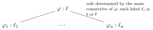
Every node carries a label , , …, dictating its status in the model under construction.
Behind these tools stands model-theoretic semantics (M-tS): fix a class of structures, define satisfaction by recursion on the connectives, and take validity to be truth in every structure. The solvers are how we often use the semantics; a tableau explores precisely the space of structures the semantics quantifies over. They are not accessories to the semantics but operationalize it. They are what makes it useful for representing and automating reasoning — for good old-fashioned AI.
An alternative semantic paradigm has recently achieved mathematical maturity: proof-theoretic semantics (P-tS) [20]. Philosophically, this approach differs from M-tS by being based on the meaning-as-use paradigm (as opposed to meaning-as-denotation) imported into logic, with use read as inferential role. Thus the word “proof” in the name should not mislead: P-tS is not proof theory, but takes inferences (rather than denotations) as primitive. The philosophical literature here is rich, but it is not our concern in this paper.
We shall concern ourselves with a particularly successful branch of P-tS known as base-extension semantics (B-eS). Here meaning is defined relative to a base: a set of inferential commitments governing atomic sentences. The meaning of a formula relative to a base is given by a judgement , called support (), whose clauses fix, for each connective, what it takes to support a formula built with it. A base may be thought of as the P-tS counterpart of a model in M-tS, and support as the counterpart of satisfaction.
The success of B-eS in recent years is its expressiveness. It has now been given for classical propositional logic [18] and for intuitionistic propositional logic (IPL) [19]; the relationship between the two is more delicate than one might expect, and we take it up in Section 3. The paradigm has since been extended to first-order logic [5], intuitionistic multiplicative linear logic [7], the logic of bunched implications [8], and modal logics [1]. Given that it has been developed for so many standard logics, the semantics should no longer be thought exotic. How does one use it though? It remains to operationalize the semantics.
So what stands to B-eS as tableaux and SAT solvers stand to M-tS? Transposing the model-search apparatus directly to B-eS would miss exactly the difference that makes the semantics interesting. The underlying idea of B-eS is behaviour, not structure. Therefore, it seems reasonable to suggest that the operational counterpart should be a search through inferential commitments (as opposed to models). Fortunately, there is already a mature technology for such search, itself a piece of good old-fashioned AI: logic programming (LP).
Our claim is not that LP may be used to implement B-eS, in the weak sense in which any mathematics can be implemented. Rather it is that LP operationalizes the unfolding of the semantics as tableaux operationalizes the unfolding of M-tS. When LP is represented as goal-directed proof-search, it decomposes a goal analogously to how tableaux decomposes a formula: the main connective of the goal determines which rule applies, disjunctive goals branch, and a branch closes successfully when the goal has been reduced to something the program supplies outright:

We write for when the search succeeds.
Since B-eS exists for many logics, the claim that it is LP has content only once the right LP language has been matched to the right logic. Here we lean on the analysis of Miller et al. [15]: a logic programming language is given by a class of definite formulae, which serve as program clauses, together with a class of goal formulae, which are queried against them, such that provability is captured by uniform proofs — goal-directed search in which the logical structure of the goal drives the computation and the program is consulted only at atoms. Horn clauses meet the requirement, and are the foundation of Prolog; so do hereditary Harrop formulae, the foundation of Prolog [14].
In this short paper, we show that the B-eS for IPL is captured by a second-order fragment of hereditary Harrop logic programming, in the family of Prolog but with quantification over atoms only. That is,
where is operational derivability and is the encoding of as a goal formula. A formula’s semantic status can be established by running it.
The correspondence pays in both directions. Read from right to left, it says that goal-directed search is not merely a proof-search discipline that happens to be complete for a well-chosen fragment: it is a semantics. A hereditary Harrop program is a meaning-conferring object rather than a database of facts, and the uniform-proof restriction is a semantic condition rather than an operational convenience.
Roadmap. Section 2 presents the three LP languages we require — Horn clauses, hereditary Harrop formulae, and their second-order extensions — with their operational semantics and a worked example. Section 3 defines support, explains its clauses, and recalls the classical/intuitionistic correspondence. Section 4 develops the encoding and proves the theorem above. Section 5 draws out the consequences and the programme they suggest. This is a short paper: apart from the cited theorems of Section 3, the definitions and results of Sections 2–4 are those of the extended version [6], where full proofs are given; we indicate the shape of the main argument as we go.
2 Logic Programming
We present LP before B-eS, since some of the machinery can then be recycled. Throughout we use a proof-theoretic presentation rather than the resolution-based approach of Kowalski [12]. The reason is flexibility: we shall consider three languages in order of increasing expressiveness. A language comprises a class of definite formulae (or clauses) and a class of goal formulae .
Definition 2.1 (Program). Let be a logic programming language. An -program is a finite set of definite formulae in the sense of .
In the proof-theoretic presentation, resolution is replaced by backchaining: to establish an atom, one looks in the program for a clause whose head is that atom. This is a change of presentation only, not of substance. A Prolog clause is thus captured by a definite clause . Here is Kowalski’s reverse implication, read “ if ”; in the grammars below we write clauses head-last, so the same clause appears as .
Definition 2.2 (Horn clauses). The language of propositional Horn clauses () consists of the definite formulae and goal formulae generated by
Observe that an implication may occur only in definite formulae, never in goals. The language can therefore express conditionals but not hypotheticals — and hypotheticals are precisely what intuitionistic logic requires. This motivates an extension in which hypothetical goals are admitted. Crucially, the extension must be such that proof-search remains goal-directed, since goal-directedness is the point of the LP formalism. The following extension is due to Miller [13] and Harland [10].
Definition 2.3 (Hereditary Harrop formulae). The language of propositional hereditary Harrop formulae (hH) is generated by
Clause heads are atomic, as in the extended version [6]: the definite formulae are those of , and the addition is in the goals. It is the hypothetical goal , whose procedural reading is: to establish under the assumption , add to the program and carry on. The program is thus no longer fixed for the duration of a computation; it grows as the search descends into implicational goals. This is the LP counterpart of discharging an assumption in natural deduction, and it is the device that will give implication its intuitionistic content.
For our systems to be genuinely operational, programs must be computable in some sense. Of course, we could simply require that they have computable descriptions — that they be recursively enumerable. However, with one small addition we can constrain the programs used throughout the paper to be finite, and hence certainly tractable for implementation. The device, following Miller et al. [15], is to observe that every program we require has a regular structure that can be captured by second-order quantification. A quantified formula packs a schematic family — one instance for each atom — into a single finite formula.
Definition 2.4 (Second-order hereditary Harrop formulae). The language extends with a second-order quantifier ranging over atoms:
Here ranges over a set of propositional variables disjoint from the atoms. The atomic formulae are the atoms together with the variables, and ranges over them in the grammars above, so that, for instance, is a definite formula. Programs and goals are closed: every variable occurring in them is bound. We write for the result of replacing the free occurrences of in by the atom , and say that an atom is fresh for a formula or program if it does not occur in it.
We have glossed the procedure as backchaining, which requires looking inside the program for clauses. Since programs in the above languages have internal structure, this inspection itself needs a procedural account. The following provides one.
Definition 2.5 (Elaboration). The elaboration of a program is defined recursively as follows:
- ;
- if , then and ;
- if , then for every atom .
Elaboration acts on clauses one at a time, so is the union of the elaborations of the members of , and in particular ; we use this freely. Note also that may be infinite, since the quantifier condition instantiates a quantified clause at every atom. This is harmless: the operational semantics inspects only finitely much of it in any one derivation. The important feature is that every clause eventually elaborates to atoms and to clauses with atomic head.
We may now say what it is to run a query. The relation is defined uniformly for all three languages, and we give the procedural reading of each clause alongside it.
Definition 2.6 (Operational semantics). The relation is defined by:
- Fact: if .
- Backchain: if and .
- And: if and .
- Or: if or .
- Augment: if .
- Generic: if for some atom not occurring in or .
Read as instructions: to establish an atom, find it in the program, or find a clause with that head and establish the clause’s body instead; to establish a conjunction, establish both parts; to establish a disjunction, choose a part and establish it; to establish an implication, assume the antecedent and continue; to establish a schematic claim, establish one instance at an atom about which nothing is known. Only the first two rules look at the program at all. The rest are determined by the goal.
Example 2.7. Let . The following query succeeds; each edge of the search tree is labelled with the rule applied.
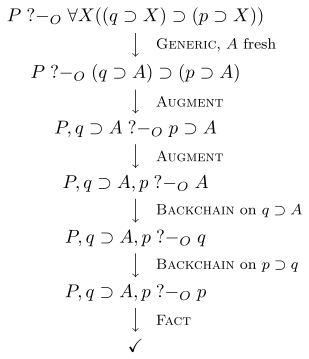
The goal expresses, schematically, that whatever follows from follows from . The fresh atom stands proxy for an arbitrary conclusion, and the two applications of Augment show the program growing as the search descends: what began as a single clause is, by the fourth line, a program of three.
The freshness condition in Generic is important. A schematic claim would seem to call for infinitely many checks, and the rule performs only one. It does not require that hold for every atom; it requires it for some atom occurring in neither the program nor the goal. Because nothing whatever is known about such an atom, a derivation using it can appeal to no property it does not share with every other atom, and so the single witness establishes the schema. This is the eigenvariable discipline of proof theory, and it is what will make the universal quantifiers of the support semantics finitary — a point on which the main theorem depends.
It remains to record three structural properties of , each of which says something one would want to be true of a search procedure. We write to mean , borrowing the notation for base extension deliberately: Section 4 will identify the two relations. All three properties are proved by routine induction on derivations, and all three preserve the height of the derivation — which matters, since the induction in Section 4 is on height.
Lemma 2.8 (Monotonicity). If and , then .
Lemma 2.9 (Renaming). Let be any function from atoms to atoms, extended homomorphically to formulae and programs. If , then .
Lemma 2.10 (Inversion). If , then . If , then for each . If , then for every atom .
Monotonicity says that adding clauses never destroys a solution. Renaming says that the names of atoms carry no information, and requires care only at Generic, where the eigenvariable must be moved out of the way of before the induction hypothesis applies; Monotonicity uses it at the same point, since the eigenvariable of a search over may occur in the larger program. Inversion is the converse of the goal-directedness we have been emphasising: because the main connective of a goal determines the last rule of its derivation — Fact and Backchain concluding only atomic goals — one can read the premisses back off the conclusion; for the quantifier, Renaming then moves the eigenvariable of Generic to any atom whatever. It is the rule-by-rule character of that makes this possible, and it is what will let the comparison with support in Section 4 run in both directions.
3 Base-extension Semantics
We have already given a brief introduction to B-eS above, and we elide further motivation in favour of the technical details. Our logical syntax is given by the grammar
with . Throughout, let be one of the LP languages of Section 2.
Definition 3.1 (Base). An -base is an -program. We write for extension of bases, meaning with an -base.
It may seem redundant to define bases and programs separately; the point is to smooth the correspondence between the two literatures. Nothing in the literature on B-eS requires bases to be finite — indeed, it is crucial that they may be infinite. The restriction to finite bases is available here only because of the second-order quantification: readers within the P-tS literature will recognise that this recovers the expressive strength required for the results cited below.
The support relation is defined relative to a fixed choice of ; the base extensions quantified over in its clauses range over -bases. Where the choice needs emphasis we speak of -support.
Definition 3.2 (Support). The relations and are defined by the clauses of Figure 1, where is a finite set of formulae and we write for .
The clauses () and () give the meaning of a connective as a consequence condition: they state what one may conclude from the formula, an atom standing proxy for an arbitrary conclusion. The formula licenses every conclusion that each disjunct separately licenses, and the formula licenses every conclusion. Each is, visibly, the elimination rule for its connective read as a definition of meaning. The clause () fits the same pattern — licenses from — expressed through the context-extension clause (Inf). The clause () is direct, but it too has an elimination form (Remark 3.3). The clause (At) is the interface with the base: atomic support is provability in the base, and here the reading of bases as programs does its first work, since is proof-search.
Remark 3.3. The clauses of Figure 1 are Sandqvist’s [19]. The direct clause for conjunction is equivalent to an elimination-style clause of the same shape as () [7]:
and implication likewise admits an elimination form: iff for every and , if and then [6, Corollary 3.7]. Every connective is thus characterised by what it licenses one to conclude.
Example 3.4. Fix . Let and consider . Does it hold? It does. Given and an atom with and , the fact yields by (At), and the first hypothesis then yields . Note that no disjunction occurs in the base: the disjunction is supported through what its disjuncts license, not through any disjunctive commitment.
A formula is -valid iff holds for every -base . Equivalently, is -valid iff . What is curious about B-eS is that the same clauses define two different logics depending on the notion of base:
Theorem 3.5 (Sandqvist [18]). A formula is -valid if and only if is provable in classical propositional logic.
Theorem 3.6 (Sandqvist [19]). A formula is -valid if and only if is provable in intuitionistic propositional logic.
Sandqvist states Theorem 3.6 for his class of bases, arbitrary sets of atomic rules of level at most two; the proof transfers unchanged to -bases [6, Section 3].
There is currently no consensus on how to understand this result. The contravariance — extends , while classical logic extends intuitionistic logic — makes some sense: in the support clauses quantify over a larger space of bases than in , so validity is harder to attain and fewer formulae achieve it. But this heuristic does not account for why one should expect exactly classical logic in the one case and exactly intuitionistic logic in the other. The key differentiating feature appears to be the hypothetical reasoning available in but not in .
Example 3.7 (Peirce’s formula). Peirce’s formula is classically valid, hence -valid by Theorem 3.5; but it is not provable in IPL, hence not -valid by Theorem 3.6. So there is a hereditary Harrop base — we shall see in Example 4.12 that the empty base suffices — at which the support clauses refuse it. The refusal is possible only because hH-extensions can install the hypothesis as a genuinely hypothetical commitment rather than a material one.
This completes our introduction to B-eS. The remainder of the paper establishes that LP, as defined above, operationalises it.
4 Soundness and Completeness
We have defined both LP and B-eS; it remains to explain their correspondence. The idea is that support judgements correspond to certain queries. Given the complexity of the clauses in Figure 1, we restrict attention to , which is expressive enough to encapsulate all the requisite structure. By Theorem 3.6, this means that in this section we are concerned only with ; classical logic is treated in Section 5.
Every LP language we consider has two syntactic classes of formula: goals, which are queried, and definite clauses, which make up the program. Roughly, these play the roles of the query and the clause database in a resolution setting, but with one crucial difference: the rule Augment, on encountering a goal , installs into the program as a hypothesis and continues with . Consequently an encoded formula may appear in either class — as a goal when it is queried, and as a program clause when Augment installs it. Since has only one class of formulae, we work with the fragment of that makes no such distinction.
Definition 4.1 (Neutral formulae). A formula is neutral if it is generated by the grammar
where ranges over atomic formulae.
Proposition 4.2. Every neutral formula is both a definite formula and a goal formula of .
The proof is a routine induction on the grammar: an implication is definite read as and a goal read as , and the remaining cases are immediate. Note that the consequent of an implication in a neutral formula is atomic: a -free implication with a compound consequent is a goal but not a definite formula.
We now encode formulae as neutral formulae.
Definition 4.3 (Encoding). To each formula , assign a formula by:
where is in each case a variable not occurring in or .
By induction on , each is neutral, so a base extended by an encoded formula is again a base. The encoding transcribes the support clauses. The goal says: for each atom taken as an arbitrary conclusion, if yields and yields , then — this is clause (), with the universal over atoms become and the quantifier over base extensions become program augmentation. The goal says that every conclusion follows. Conjunction is encoded directly, following clause (). Implication is encoded in elimination form: the goal says that, for an arbitrary conclusion , together with the continuation yields — the elimination form of () recorded in Remark 3.3. The direct encoding is the natural first thought, but its consequent is in general compound, so it is not a definite formula and cannot be installed in a base by Augment; the elimination form keeps every clause head atomic [6]. The image of the encoding uses only atoms, , , and : the goal-only connective never occurs.
Remark 4.4 (Nomenclature). Definitions of the connectives from and a propositional quantifier go back to Russell, and their proof-theoretic study to Prawitz; the encoding is accordingly the Russell–Prawitz translation of the connectives [17, 16], here with the quantifier restricted to atomic instantiation as in the atomic polymorphism literature [2, 3] (see also Remark 4.6). Functional programmers will recognise the shape of a continuation-passing transform — the atom is a continuation, an arbitrary conclusion to be delivered — and we retain that reading informally, but we do not call the encoding CPS: the term has a precise, and different, meaning as a transformation on source programs.
Remark 4.5. The encoding is not one clever translation among many. It is determined, connective by connective, by the support semantics: conjunction is transcribed from its clause directly, and , , and from their elimination behaviour, by replacing the quantifier over atoms with and the quantifier over base extensions with . This canonicity suggests an explanation of the coincidence observed in [4] between Mints’ clausal translation of IPL and Sandqvist’s completeness construction: both are arrived at by writing the elimination rules as clauses over atomic vocabularies — instances of the same Russell–Prawitz transcription, reached from different directions.
Before proving the encoding faithful, it is worth asking how neutral formulae sit within LP. Atoms are the paradigm of a formula that is simultaneously a goal and a definite clause, and neutral formulae extend that class; so one might expect them to behave like atoms in every respect — in particular, to be substitutable for them. They are not, and the reason is instructive.
In full second-order propositional logic a universal quantifier may be instantiated at an arbitrary formula. The quantifier of is not of this kind: operationally it is atomic. Generic discharges a universal goal by introducing a single fresh atom, and elaboration instantiates a universal clause only at atoms. This restriction is what keeps proof search effective, and it is exactly what separates neutral formulae from atoms.
Remark 4.6 (Failure of compound instantiation). It is tempting to posit the following substitution principle: if and the atom does not occur in , then for every neutral . It fails. Take
where , , and are distinct atoms.
The atomic instance succeeds. Augment turns into the query . As is an atom, is an instance of the clause of and so lies in the elaboration ; Backchain on it leaves , which Fact closes.
The compound instance fails. Substituting for yields the goal , and after Augment the query . Since the clause of elaborates at atoms only, the clauses of with head are precisely those of the form with atomic, so Backchain demands that some atom be derivable. None is: the only heads available are , which itself requires an atom, and , which requires . Hence .
Atomic polymorphism. By Generic, the successful half says precisely that . So the universal goal is derivable while one of its compound instances is not: the quantifier of is genuinely atomic. This is the operational face of the predicativity of atomic polymorphism [2], and it carries a methodological consequence. Theorem 4.9 cannot be proved by a substitution lemma. The arguments below use instead renaming (Lemma 2.9), which replaces atoms by atoms, together with identity and cut for neutral formulae.
Nonetheless, some of the behaviour of atoms does survive, and it is exactly the behaviour proof search relies on. The rule Fact, which closes an atomic goal sitting in the elaborated program, generalises to neutral formulae; so does the admissibility of cut.
Lemma 4.7 (Identity). Let be neutral. If , then . In particular, for every program .
Lemma 4.8 (Cut). Let be neutral. If and , then .
Note that neither statement would even typecheck without Proposition 4.2: in each, occurs once as a goal and once as a program clause. This is where membership in both syntactic classes earns its keep.
Identity is proved by induction on the size of , where has the same size as . Cut is proved by induction on the size of and, within it, on the height of the derivation of . Its key step is that every member of is neutral, of size at most that of , and derivable from whenever is, by inversion (Lemma 2.10); renaming (Lemma 2.9) handles the eigenvariable introduced by Generic. The arguments are those of cut-admissibility for uniform proofs [15], adapted to the atomic quantifier. Details are in the extended version [6].
We can now return to the picture from the introduction. A tableau decomposes a formula according to its main connective; goal-directed search decomposes a goal in the same way. The encoding of Definition 4.3 makes the two decompositions line up with a third: the clauses of Figure 1. Each connective of IPL is sent to a neutral formula whose outermost structure determines which rule of fires, and that rule re-enacts the support clause for that connective. Conjunction is sent to , where And splits the goal. Falsum is sent to , where Generic introduces a fresh atom to be derived. Implication and disjunction are sent to universal formulae, where Generic introduces a fresh atom, Augment installs the continuation clauses just as the support clauses quantify over base extensions, and Backchain consumes them.
Theorem 4.9 (Soundness and Completeness). For every base and IPL formula :
Proof sketch. By simultaneous induction on , both directions together. The case of atoms is clause (At). For , Generic at an atom fresh for gives one direction and inversion the other. For , clause (), the induction hypothesis, And, and inversion suffice. For and , left to right: Generic and Augment reduce the encoded goal to proving a fresh atom from , where is the continuation clause — for , and for . For , the induction hypothesis and Backchain on give for each , and clause () delivers . For , identity and the induction hypothesis give , clauses () and (Inf) give , and the induction hypothesis and Backchain on give . Right to left: given the extension and atom supplied by clause (), or by the elimination form of () (Remark 3.3), monotonicity and inversion unwind Generic and Augment to give ; identity, the induction hypothesis, Augment, and And give ; and cut gives . Since the induction hypothesis is used in both directions, the two are proved together. Compound instantiation is never used, in keeping with Remark 4.6: the fresh atom of Generic is moved to the atom supplied by the support clause by inversion, which is to say by renaming. The full proof is [6, Theorem 4.2]. □
Corollary 4.10. is valid in IPL if and only if .
Example 4.11. The formula encodes as , since . The query succeeds from the empty program:
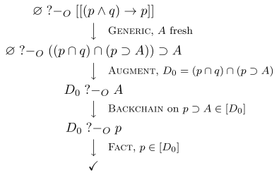
The fresh atom is the conclusion to be delivered. Backchaining passes control to the continuation , and the conjunct is then found in the elaborated program: the elimination rule for conjunction is executed as a projection.
Example 4.12 (Peirce’s formula, executed). Write and , so that . The search from the empty program runs as follows:
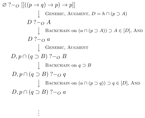
The alternatives lead to the same place. At the second line, Backchain on demands , and the only clauses with head are instances of , which demand ; at the fourth, Backchain on the instance of at demands directly. So every branch returns to the goal , and establishing requires , whose only clauses are instances of demanding again. Any derivation would therefore contain a strictly shorter one of the same kind, so there is none: , which by Corollary 4.10 witnesses the intuitionistic invalidity of Peirce’s formula — and, by Theorem 4.9, the failure of support at the empty base promised in Example 3.7. The formula is classically valid; what the failed search records is that the hypothesis , installed as a genuinely hypothetical commitment, yields only given , and nothing yields .
This operationalizes the B-eS for IPL. We motivated it as the analogue of tableaux for P-tS, and before closing the section that motivation merits some final remarks. The analogy breaks in three places, but each break is the M-tS/P-tS difference showing through.
First, polarity. Every node of a tableau carries a label or , recording the status the formula is to have in the model under construction; the search is a refutation, begun by supposing false. A query carries no such label. There is nothing to suppose false, because support is not truth-in-a-structure and its negation is not a constraint one can propagate. The search is direct: it looks for the commitments that would confer the meaning, not for a structure witnessing that they fail.
Second, and consequently, the two searches read their branches dually. A tableau succeeds by closing every branch and refutes by leaving one open, the open branch being the countermodel it has built. Goal-directed search succeeds on a single branch and fails only when no branch can close; and when it fails it hands back nothing. Example 4.12 produces no object witnessing the failure of support — only the observation that every branch returns to the same unmet demand. In M-tS a refutation must exhibit a structure, since validity is truth in all of them. Here the base is given in advance, and the quantification over extensions has been absorbed into the support clauses themselves. There is no countermodel to build because there is nothing left to construct.
Third, the program grows. Augment installs a hypothesis and the search continues against a larger program, so the object consulted at the leaves is not fixed in advance. A tableau branch also grows, but it grows by decomposition: what appears is always a subformula of what was there. This is what Example 4.12 turns on. Peirce’s formula fails not because some branch stays open, but because the hypothesis , once installed as a genuine commitment, licenses nothing that can be discharged.
None of this is a defect of the analogy; it is the analogy doing its work. We should not expect the operationalization of a use-based semantics to look like the operationalization of a denotational one, and the respects in which the two differ are exactly the respects in which B-eS differs from M-tS. What survives is the structural claim with which we began: a rule determined by the main connective, branching where the connective demands a choice, and closure when the decomposition reaches something the ambient object supplies outright. That claim survives intact, and Corollary 4.10 shows it survives with something to spare. Validity in M-tS is a quantification over structures, which a tableau discharges by constructing the one candidate that matters. Validity here is a single query against the empty program. The quantifier that a tableau must simulate has already been paid for by the semantics.
5 Extensions and classical logic
We have established the operationalization only for the B-eS of IPL, but such semantics now exist for a range of logics: first-order logic [5], linear logic [7], the logic of bunched implications [8], and modal logics [1]. In each case the support clauses have the shape that drove the present construction — a quantification over base extensions, discharged at atoms. The programme this paper suggests is accordingly: for each such logic, find the LP language whose operational steps internalise those quantifiers. The expected pairings are informative — first-order B-eS with first-order hereditary Harrop programs [15, 10], IMLL with the linear hereditary Harrop programs of Lolli [11] — and the first-order case is the natural first test, both sides of the correspondence being already in place.
In every case the challenge is one of expressiveness, and classical logic shows what is at stake. Theorem 3.5 identifies B-eS over with classical logic, so the target language is fixed for us; but the encoding of Definition 4.3 cannot live there. Its work is done by — a continuation abstracted over, then supplied — and while has the quantifier, it has no hypothetical goals, so neither the goal nor its body is available there. The pairing that Theorem 3.5 hands us is therefore the one pairing for which we have no encoding, and the machinery that made IPL work is exactly what withholds.
Classical validity, on the other hand, is already within reach. By Glivenko’s theorem, is classically valid if and only if is intuitionistically valid, so by Corollary 4.10 it suffices to run
But this is a reduction, not an operationalization. It decides classical validity by running an intuitionistic query, and so tells us nothing about how a classical base confers meaning; the double negation is a device of the translation rather than anything the search enacts. It also does not travel: Glivenko’s theorem is propositional, so the route closes precisely where the programme above says to go next.
A native treatment would have to make the classical structure operational rather than translate it away, and the continuation reading suggests where to look. In the typed -calculus, continuations at classical type are control operators [9], which points to an operational semantics with a control facility — a restart, or a backtracking-to-continuation rule — layered over Horn programs. This would keep the program language that Theorem 3.5 demands while recovering operationally the expressive power the encoding obtained from . Whether the resulting notion of success matches support over a Horn base is the obvious question, and we leave it open.
References
- [1]
- Timo Eckhardt and David J Pym. Base-extension Semantics for Modal Logic. Logic Journal of the IGPL, 33, 2024. doi:10.1093/jigpal/jzae004.
- [2]
- Fernando Ferreira. Comments on Predicative Logic. Journal of Philosophical Logic, 35(1):1–8, 2006.
- [3]
- Fernando Ferreira and Gilda Ferreira. Atomic Polymorphism. The Journal of Symbolic Logic, 78:260–274, 2013.
- [4]
- Alexander V. Gheorghiu. On an Inferential Semantics for Intuitionistic Sentential Logic. Journal of Logic and Computation, 35(4), 2025.
- [5]
- Alexander V. Gheorghiu. Proof-theoretic Semantics for First-order Logic. Logic Journal of the IGPL, 33(5), 2025.
- [6]
- Alexander V. Gheorghiu. Support is search. arXiv:2603.13018, 2026.
- [7]
- Alexander V. Gheorghiu, Tao Gu, and David J. Pym. Proof-theoretic Semantics for Intuitionistic Multiplicative Linear Logic. In Revantha Ramanayake and Josef Urban, editors, Automated Reasoning with Analytic Tableaux and Related Methods — TABLEAUX, pages 367–385. Springer, 2023.
- [8]
- Alexander V. Gheorghiu, Tao Gu, and David J. Pym. Proof-theoretic Semantics for the Logic of Bunched Implications. Studia Logica, 2025.
- [9]
- Timothy G. Griffin. A formulae-as-types notion of control. In Proceedings of the 17th ACM SIGPLAN-SIGACT Symposium on Principles of Programming Languages (POPL ’90), pages 47–58. ACM, 1990.
- [10]
- James Harland. On Hereditary Harrop Formulae as a Basis for Logic Programming. PhD thesis, University of Edinburgh, 1991.
- [11]
- Joshua S. Hodas and Dale Miller. Logic programming in a fragment of intuitionistic linear logic. Information and Computation, 110(2):327–365, 1994.
- [12]
- Robert Kowalski. Logic for Problem Solving. Number 7 in Artificial Intelligence Series. North-Holland, New York, 1979.
- [13]
- Dale Miller. A Logical Analysis of Modules in Logic Programming. The Journal of Logic Programming, 6(1-2):79–108, 1989.
- [14]
- Dale Miller and Gopalan Nadathur. Programming with Higher-Order Logic. Cambridge University Press, Cambridge, 2012.
- [15]
- Dale Miller, Gopalan Nadathur, Frank Pfenning, and Andre Scedrov. Uniform proofs as a foundation for logic programming. Annals of Pure and Applied logic, 51(1-2):125–157, 1991.
- [16]
- Dag Prawitz. Natural Deduction: A Proof-theoretical Study. Dover Publications, 2006 [1965].
- [17]
- Bertrand Russell. The Principles of Mathematics. Cambridge University Press, Cambridge, 1903.
- [18]
- Tor Sandqvist. Classical Logic without Bivalence. Analysis, 69(2):211–218, 2009.
- [19]
- Tor Sandqvist. Base-extension Semantics for Intuitionistic Sentential Logic. Logic Journal of the IGPL, 23(5):719–731, 2015.
- [20]
- Peter Schroeder-Heister. Proof-Theoretic Semantics. In Edward N. Zalta, editor, The Stanford Encyclopedia of Philosophy. Metaphysics Research Lab, Stanford University, Spring 2018 edition, 2018.
University College London
Email address: [email protected]