COMP0009 Logic, Chapter 7: SAT Solving

Gheorghiu, Alexander V.

The completeness theorem for $NK$ , Gentzen’s natural deduction with the law of the excluded middle, says that whenever a sentence follows from others, it has a derivation from them. It says nothing about how to find the derivation, and finding one can be hard. At every step there could be an instance of excluded middle for every formula one could think of, and a choice of term for every quantifier, and nothing on the page says which choice leads anywhere. So how does one check whether a given sentence $φ$ is entailed by a set $Γ$ of sentences?

The proof of the completeness theorem contains a suggestion. It builds a model of $Γ \cup {\neg φ}$ out of a failure to derive $φ$ from $Γ$ . So instead of searching for a derivation of $φ$ from $Γ$ , we may search for such a model. If there is one, it shows that $φ$ does not follow from $Γ$ ; if the search shows that there is none, then $φ$ does follow. This idea has been one of the most effective in automated reasoning.

In the end the search comes down to something very simple. As far as the question is concerned, a structure is pinned down by which basic facts hold in it: whether this element has that property, whether those two are related. Think of each basic fact as a switch, on when the fact holds in the structure being built and off when it does not. Building a model is then choosing a setting of the switches, one that makes every sentence true, and the programs that search for such a setting are called SAT solvers, SAT for satisfiability.

SAT solvers are among the most used tools of logic. Whenever a problem comes down to “find a choice of yes-or-no settings that obeys all these constraints, or show that there is none”, a solver can be put to work on it, and many problems do.

Hardware. Chip makers check that an optimised circuit computes the same function as its specification, and search for inputs that drive a design into a bad state within a given number of clock cycles. A bug found this way costs nothing; one found after manufacture can cost a fortune.
Software. Questions about programs (can this index go out of bounds? can these two versions of a function ever disagree? can anyone outside this account read this file?) are translated into satisfiability questions, usually through the SMT solvers of Remark 7.37, which run a SAT solver at their core.
Configuration. Installing software means choosing versions of packages so that every dependency is met and no two conflict, and several package managers hand that problem to a SAT solver. Configuring a product with options that exclude or require one another is the same problem.
Planning and scheduling. Timetables, rosters and plans are written as “at each step, which actions happen”, and the solver finds a plan or shows that none exists.
Mathematics. Solvers have settled open combinatorial questions by exhaustive search, among them the Boolean Pythagorean triples problem in 2016, with a certificate of some two hundred terabytes that an independent program checked.

In none of these does anybody write the solver’s input by hand. The problem is stated in a natural language of its own, with quantifiers and arrows and arithmetic, and a program translates it into the shape the solver wants. This chapter studies both halves: the translation and the search.

Here is the search in miniature. Suppose you want to know whether some constraints entail a claim, and a derivation will not come: at every step there is a guess to make, and nothing says which guess leads anywhere. Treat the question as you would a bug, and ask what a counterexample would look like. Suppose the claim fails, and give the “someone” who breaks it a name. Then read the constraints against what you have written, one named thing at a time, and write down what they force. Either the page collapses, with every line forced by the lines above it, and the constraints entail the claim; or the demands run out, and what is left on the page is a structure in which the constraints hold and the claim fails: a counter-model, which serves as a bug report. Example 7.4 runs this search on an access policy, twice.

The chapter asks four questions about such a search:

Why is a search for a counter-model as good as a proof?
How does a machine search for a setting of the switches, and what certifies its answer?
Why may the search look only at the things it has named?
Does the search always come to an end?

The chapter answers them by first solving a simpler problem, with no quantifiers at all (given constraints on finitely many switches, is there a setting that obeys them?), and then reducing the first-order problem to it.

Section 7.1 turns entailment into the question whether a set of sentences has a model.
Section 7.2 fixes one shape for constraints, the clause, which forbids some settings of the switches.
Section 7.3 solves the simpler problem with DPLL, and certifies the answer either way.
Section 7.4 gives every “someone” a name and turns sentences into clauses.
Section 7.5 proves that the names are enough.
Section 7.6 hands the instances, level by level, to DPLL.

Two optional sections follow: Section 7.7 opens the black box of Section 7.4, and Section 7.8 shows that a failed search is itself a proof, that some such proofs must be long, and how the instances that can clash are found without listing the rest. The main line quotes some of their results but none of their proofs. The History at the end tells who did what.

7.1 Satisfiability

This section turns the question we started from, whether a set $Γ$ of sentences entails a sentence $φ$ , into the question that a solver answers: whether a set of sentences has a model. Throughout, $Σ$ is a signature, and structures and sentences are $Σ$ -structures and $Σ$ -sentences.

A sentence can be true in one structure and false in another, and the words we need sort sentences by the structures that make them true. A sentence $φ$ is

true in a structure $M$ if $M ⊨ φ$ ;
valid if it is true in every structure;
contingent if it is true in some structures and false in others.

Satisfiability, the case that matters here, gets a definition of its own. A programmer may read $φ$ as a test and a structure as an input: then $φ$ is satisfiable when some input passes the test, and valid when every input does.

Definition 7.1 (satisfiable). A sentence, or a set of sentences, is satisfiable if some structure makes it true.

Formally, a $Σ$ -sentence $φ$ is satisfiable if $M ⊨ φ$ for some $Σ$ -structure $M$ , and unsatisfiable otherwise. A set $Γ$ of $Σ$ -sentences is satisfiable if it has a model, that is, if some $Σ$ -structure $M$ satisfies it, $M ⊨ Γ$ , and unsatisfiable otherwise.

Three confusions are easy to make, and the definitions rule each of them out.

A sentence true in a structure need not be valid: another structure may make it false.
A satisfiable sentence need not be true in the structure one has in mind.
A sentence that is not valid need not be unsatisfiable: a contingent sentence and its negation are both satisfiable.

Example 7.2 (the company: eight sentences). Harriet Ashworth looks after the platform of the company of Chapter 6, and the company is her structure $C$ : Tuesday’s personnel table, in the company signature. Figure 7.1 classifies eight sentences of the company signature, with the evidence for each verdict.

Sentence	Verdict	Evidence
$Eng (ceo) \lor \neg Eng (ceo)$	valid	in every structure one disjunct is true
$(\forall x Eng (x)) \to Eng (ceo)$	valid	whatever $ceo$ names is one of everything
$\forall x (Eng (x) \to Mgr (boss (x)))$	contingent	true in the company; false in a one-person company whose chief executive is an engineer and not a manager
$Richer (ceo, ceo)$	contingent	false in the company; true when $Richer$ is interpreted as ${(d, d) : d \in D}$
$(\exists x Mgr (x)) \to \forall x Mgr (x)$	contingent	true in a company of managers; false in the company
$\neg \forall x Eng (x)$	contingent	true in the company; false in a company of engineers
$\exists x Eng (x) \land \forall x \neg Eng (x)$	unsatisfiable	the first conjunct needs an engineer, the second forbids one
$\forall x Mgr (x) \land \neg Mgr (ceo)$	unsatisfiable	whatever $ceo$ names would be a manager and not one

Figure 7.1. Eight sentences of the company signature.

The table shows each of the three confusions at work.

The policy $\forall x (Eng (x) \to Mgr (boss (x)))$ holds in the company, and a company with different staff can break it.
The sentence $Richer (ceo, ceo)$ is satisfiable, though no sensible company makes it true: nothing in the signature says that $Richer$ comes from salaries.
The sentence $\neg \forall x Eng (x)$ is not valid, and neither is its negation, so both are satisfiable.

The evidence for such verdicts comes in two kinds. A verdict that something happens in some structure (satisfiable, or not valid) is backed by a single structure, and anyone can check it by evaluating the sentence there. A verdict that something happens in every structure, or in none (valid, or unsatisfiable), is backed by an argument that speaks of all structures at once, and no evaluation checks an argument of that kind (the third column of Figure 7.1 has both). This chapter produces the second kind of evidence by searching for the first.

Now the question we started from, whether $Γ ⊨ φ$ . The entailment fails exactly when some model of $Γ$ makes $φ$ false, and then a single model, evidence of the first kind, shows it. Such a model has a name.

Definition 7.3 (counter-model). A counter-model is a structure that shows an entailment to fail.

Formally, a counter-model to $Γ ⊨ φ$ is a model of $Γ$ in which $φ$ is false, that is, a structure $M$ with $M ⊨ Γ$ and $M ⊭ φ$ .

By the definition of entailment, either $Γ ⊨ φ$ holds or it has a counter-model.

Example 7.4 (the company, cont’d: a policy change and a bug report). Harriet has been asked to sign off a change to the company’s access policy. Two rules have been proposed, that engineers report to managers and that managers are not engineers:

\begin{aligned} P_{1} & : \forall x (Eng (x) \to Mgr (boss (x))), \\ P_{2} & : \forall x (Mgr (x) \to \neg Eng (x)) . \end{aligned}

Their point is that no engineer ever reports to another engineer:

C : \forall x (Eng (x) \to \neg Eng (boss (x))) .

Do $P_{1}$ and $P_{2}$ entail $C$ ? Forty minutes on a derivation in $NK$ leave Harriet with a page of guesses, so she asks what a counterexample would look like. Suppose some engineer, call her $a$ , reports to an engineer. By $P_{1}$ , $a$ ’s boss is a manager. By $P_{2}$ , $a$ ’s boss is not an engineer. But $a$ ’s boss is an engineer, and every line was forced by the lines above it. No company obeying the two rules contains such an $a$ : the rules entail the claim.

The same afternoon a colleague proposes dropping $P_{2}$ , so that a senior engineer can lead a team. Harriet runs the same search. Suppose an engineer $a$ reports to an engineer $b$ . By $P_{1}$ , $b$ is a manager, and now nothing forbids a manager from being an engineer, so nothing collapses. By $P_{1}$ again, $b$ ’s boss must be a manager, and the simplest choice is $b$ herself, as the personnel table does for the chief executive. The demands run out, and what is left on the page is a structure: two engineers, with $b$ a manager and the boss of both. It obeys $P_{1}$ and breaks $C$ at $a$ . That is a bug report, not a failed proof: it says what the weakened policy allows, an engineer who manages an engineer.

So the two-person company is a counter-model to ${P_{1}} ⊨ C$ , once the symbols that the sentences do not mention are given a meaning:

$ceo$ names $b$ ;
$Richer$ is empty;
$=$ is identity.

Two people are not the smallest counter-model: Example 7.66 finds one with a single person. There is none for ${P_{1}, P_{2}} ⊨ C$ , as the first search showed.

Lemma 7.5 (reduction to satisfiability). For every set $Γ$ of sentences and all sentences $φ$ and $ψ$ :

$Γ ⊨ φ$ if and only if $Γ \cup {\neg φ}$ is unsatisfiable;
$φ$ is valid if and only if $\neg φ$ is unsatisfiable;
$φ$ and $ψ$ are true in the same structures if and only if $(φ \land \neg ψ) \lor (ψ \land \neg φ)$ is unsatisfiable.

Proof. A model of $Γ \cup {\neg φ}$ is a model of $Γ$ in which $φ$ is false, since $\neg φ$ is true exactly when $φ$ is not; that is, a counter-model to $Γ ⊨ φ$ . So (i) says that an entailment holds exactly when it has no counter-model, which is the definition. Part (ii) is (i) with $Γ$ empty, and (iii) is Exercise 7.1. □

In words: every question about what follows from what, about validity and about saying the same thing is a question about whether some set of sentences has a model.

The lemma is nearly a tautology (in classical logic, where $\neg φ$ is true exactly when $φ$ is not), and its use lies in what it suggests. A proof that $Γ ⊨ φ$ can be a failed search: try to build a model of $Γ \cup {\neg φ}$ , and show that every way of doing so collapses. This is why a search for a counter-model is as good as a proof.

So the question to hand to a program is whether a set of sentences, such as $Γ \cup {\neg φ}$ , has a model. A program can only be handed finitely many sentences, so from now on such a set is finite. We call the members of the set its constraints, since each is a sentence that the model being sought must make true.

A program that decides whether a finite set of constraints has a model is a solver. We want it to give evidence for its verdict as well as the verdict itself, evidence that can be checked without trusting the solver.

When the answer is “yes, $Γ \cup {\neg φ}$ has a model”, the evidence is a structure that satisfies the set. When the structure is finite, anyone can check it by evaluating the sentences in it.
When the answer is “no, $Γ \cup {\neg φ}$ has no model”, the evidence has to be a finite object that shows every attempt to build a model collapsing. Section 7.3 builds one.

How is a solver to search for a model? It cannot go through the structures one by one: a structure that satisfies the constraints may have five elements, or be the natural numbers, or the real line, and there is no list of them to go through. A search by hand does something narrower. It names the things it needs, and records for each basic fact about them whether the fact holds. A basic fact of this kind is an atomic sentence about named things, such as $Eng (a)$ or $Mgr (boss (a))$ , and the structure being built either makes it true or makes it false.

So each atomic sentence works as a switch, on or off, and what the search builds is a setting of the switches: a choice of on or off for each of them. A setting is something a program can handle. It can be written down; finitely many switches have finitely many settings; and a search through them can be seen to have failed. This is why a solver searches for a setting rather than for a structure. Section 7.5 shows that nothing is lost by doing so: a set of constraints has a model exactly when some setting of the switches about its names obeys every instance of the constraints at those names.

To reach the switches, the constraints have to be rewritten, and one of the rewritings brings in new symbols. A search that gives the “someone” of a negated claim a name, $a$ , has brought in a new symbol. A rewritten set that mentions symbols the original does not is not true in the same structures as the original. What a rewriting must keep is the solver’s verdict: the new set must have a model exactly when the old one does. That property has a name.

Definition 7.6 (equisatisfiable). Two sets of sentences are equisatisfiable when both have a model or neither does.

Formally, sets $Γ$ and $Δ$ of sentences are equisatisfiable if $Γ$ is satisfiable exactly when $Δ$ is.

In words: for the purpose of the verdict, one set may stand in for the other. The notion is weaker than being true in the same structures. The sets ${\exists x P (x)}$ and ${P (a)}$ , for a one-place relation symbol $P$ , are equisatisfiable, since both have models; but in a structure with two elements, only one of them in $P$ , with $a$ naming the other, the first is true and the second false. Weaker is what we want, since it leaves room for exactly this kind of rewriting: naming a “someone”, or adding new symbols of any other kind, as long as the verdict survives.

Equisatisfiability is enough for the verdict, but not for the evidence. When the answer is yes, the solver returns a structure that satisfies the rewritten set $Δ$ , and what we asked for was one that satisfies the original set $Γ$ . The definition alone does not give one. The sets ${P (a)}$ and ${Q (a)}$ are equisatisfiable, since both have models, but a structure that satisfies the second, in which $a$ names an element of $Q$ , need not satisfy the first, in which it names an element of $P$ . A solver that rewrote the first set into the second would give the right verdict and evidence for the wrong question.

So each rewriting in this chapter comes with a way back: a way of turning every structure that satisfies $Δ$ into one that satisfies $Γ$ . For the naming of a “someone” the way back is simply to forget the name, as the theorem on the clause form in Section 7.4 shows.

7.2 Clauses

Section 7.1 turned the question whether $Γ ⊨ φ$ into the question whether $Γ \cup {\neg φ}$ has a model. This section and the next solve that question for constraints without quantifiers; the quantifiers wait until Section 7.4, and nothing is lost by setting them aside, since once they have been dealt with every constraint is of the kind treated here. This section rewrites every constraint as a set of clauses, lists of switches each set on or off, of which at least one must hold.

Without quantifiers, a constraint is built from atomic sentences, such as $Eng (a)$ and $Mgr (boss (a))$ , by the connectives, and whether it is true in a structure depends only on which of its atomic sentences are true there. What is inside an atomic sentence plays no part. The sentence $Eng (boss (a))$ might as well be a single letter, $p_{Eng (boss (a))}$ say, that is either true or false: one switch.

So in this section we simplify the language. We fix a set $P$ of letters (the atomic sentences of a signature, say, each read as one letter), write $p$ , $q$ , $r$ for letters, and build formulas by the grammar

φ, ψ ::= p ∣ ⊥ ∣ \neg φ ∣ (φ \to ψ) ∣ (φ \land ψ) ∣ (φ \lor ψ),

where $p \in P$ , with the bracket conventions of Chapter 6 and with $⊤$ abbreviating $\neg ⊥$ . In this section the constraints are these formulas. Logic about letters alone is called propositional logic, as opposed to the predicate logic of Chapter 6, whose atomic formulas take arguments.

One choice here departs from Chapter 6, on purpose. There $\neg φ$ abbreviated $φ \to ⊥$ ; here $\neg$ is a connective in its own right. The two readings always give $\neg φ$ the same truth value, so nothing is lost. What is gained is that the translations below can say directly what they do to a negation.

Definition 7.7 (valuation). A valuation sets each switch on or off, and so makes each formula true or false.

Formally, a valuation is a function $v : P \to {true, false}$ . It is extended to formulas by recursion on the shape of the formula:

v (φ) : = {\begin{cases} v (p) & if φ is p, \\ false & if φ is ⊥, \\ not v (ψ) & if φ is \neg ψ, \\ v (ψ) and v (χ) & if φ is ψ \land χ, \\ v (ψ) or v (χ) & if φ is ψ \lor χ, \\ (not v (ψ)) or v (χ) & if φ is ψ \to χ, \end{cases}

where $not$ , $and$ and $or$ are the operations on ${true, false}$ given by their truth tables: $not x$ is true exactly when $x$ is false, $x and y$ exactly when both are true, and $x or y$ exactly when at least one is.

In words: a valuation is a row of a truth table, and $v (φ)$ is the entry of $φ$ in that row. A program computes it as a circuit computes its output, gate by gate from the inputs.

Definition 7.8 (satisfaction by a valuation). A valuation satisfies a formula when it makes the formula true, and a set of formulas when it makes every member true.

Formally, let $v$ be a valuation. Then $v$ satisfies a formula $φ$ , written $v ⊨ φ$ , if $v (φ) = true$ ; and $v$ satisfies a set $Γ$ of formulas, written $v ⊨ Γ$ , if $v ⊨ ψ$ for every $ψ \in Γ$ .

Definition 7.9 (satisfiable set of formulas). A set of formulas is satisfiable when some row of the truth table makes all of it true.

Formally, a set $Γ$ of propositional formulas is satisfiable if $v ⊨ Γ$ for some valuation $v$ , and unsatisfiable otherwise.

The words are those of satisfaction in a structure, on purpose. A structure for a signature of letters amounts to a valuation (Proposition 6.28), and then $v (φ) = true$ says exactly what $M ⊨ φ$ says.

The rewritings of this section must not change which settings a constraint allows, and the next definition says what that means.

Definition 7.10 (equivalent formulas). Two formulas are equivalent when they take the same value in every row of the truth table.

Formally, formulas $φ$ and $ψ$ are equivalent, written $φ \equiv ψ$ , if $v (φ) = v (ψ)$ for every valuation $v$ .

The symbol $\equiv$ is not a connective. Like $⊨$ , it states a fact about formulas from outside the language, and $φ \equiv ψ$ is not itself a formula. Equivalence is a congruence: replacing a part of a formula by an equivalent part gives an equivalent formula, since $v$ computes the value of a formula from the values of its parts. Every rewriting in this section replaces a formula by an equivalent one, and that is what entitles us to treat a constraint as nothing more than its truth table.

Remark 7.11 (Boolean algebra). The two truth values with $not$ , $and$ and $or$ form the smallest Boolean algebra, and they obey the laws that algebra is known for: $and$ and $or$ are commutative and associative, each distributes over the other, $not$ undoes itself, and $not$ turns $and$ into $or$ and back. Each law can be checked in a few rows of a truth table, and each is an equivalence.

A constraint, as the word suggests, forbids. When we care about deduction, what matters in a formula is how its parts are connected. When we care only about the switches, what matters is which settings the formula allows, and a constraint is nothing more than the settings it rules out. Take

φ : = p \land q \to r,

read “if $p$ and $q$ are on, then $r$ must be on”. Its truth table has eight rows:

\begin{array}{cccc} p & q & r & p \land q \to r \\ T & T & T & T \\ T & T & F & F \\ T & F & T & T \\ T & F & F & T \\ F & T & T & T \\ F & T & F & T \\ F & F & T & T \\ F & F & F & T \end{array}

Only one row has F, the one with $p$ on, $q$ on and $r$ off. As a constraint on valuations, $φ$ says no more than “never $p$ on, $q$ on and $r$ off at the same time”.

That is all a constraint can ever do. Its value is fixed by the values of its letters and by nothing else, so it can only rule out combinations of on and off. To rule out “ $p$ on, $q$ on, $r$ off” is to demand that at least one switch differ from it: $p$ off, or $q$ off, or $r$ on. So the constraint becomes

\neg p \lor \neg q \lor r .

Each disjunct names one switch and says whether to $p$ or not to $p$ , and at least one of them must be obeyed. A constraint that rules out several settings becomes several such disjunctions, one for each. This is the shape we want every constraint in, and the rest of the section makes it precise.

Definition 7.12 (literal). A literal says one thing about one switch: that it is on, or that it is off.

Formally, a literal is a letter $p$ or a negated letter $\neg p$ . We write $ℓ$ for a literal, and $\bar{ℓ}$ for its complement: $\bar{p}$ is $\neg p$ , and $\overset{―}{\neg p}$ is $p$ .

For instance, $\neg q$ is a literal with complement $q$ , while $\neg \neg q$ and $p \land q$ are not literals.

Definition 7.13 (clause, clause set). A clause is a constraint in its plainest shape: a list of literals of which at least one must hold.

Formally, a clause is a finite set of literals, written as the disjunction $ℓ_{1} \lor \dots \lor ℓ_{n}$ of its members; the empty clause, with no literals, is written $◻$ . A clause set is a finite set of clauses, written, when it helps, as the conjunction $C_{1} \land \dots \land C_{m}$ of its members. We write $C$ , $D$ for clauses and $S$ for clause sets.

In words: a clause is an “at least one of these”, and a clause set is a list of such demands. Since a clause is a set, neither the order of its literals nor repetition matters: $p \lor q$ , $q \lor p$ and $p \lor q \lor p$ are the same clause. A clause with one literal is a unit clause.

Read as a disjunction and a conjunction, a clause and a clause set are formulas, and satisfaction needs no new definition. A valuation satisfies a clause when it makes one of its literals true, and a clause set when it satisfies every clause in it. So nothing satisfies the empty clause, which has no literal to make true, and everything satisfies the empty clause set, which makes no demand. A clause set is the switchboard made precise: a list of demands, each of which some switch must meet.

Example 7.14 (the platform: five rules). Harriet’s platform has a hundred feature switches, each on or off, and a file of rules that the switches must obey together. Three of its switches are fast-sync, offline-mode and compression, which we write as the letters $p$ , $q$ and $r$ , and five rules in the file concern them.

fast-sync needs offline-mode, since a fast sync resumes from the offline cache.
offline-mode needs fast-sync, since the cache is filled by fast syncs.
The mobile app needs fast-sync or offline-mode; with neither it cannot work at all.
With both fast-sync and offline-mode on, compression must be on, or the sync saturates the link.
With both fast-sync and offline-mode on, compression must be off, since the offline cache cannot read compressed packets.

As clauses, with the pattern each forbids beside it:

\begin{aligned} C_{1} & = \neg p \lor q & never p on, q off; \\ C_{2} & = \neg q \lor p & never q on, p off; \\ C_{3} & = p \lor q & never p off, q off; \\ C_{4} & = \neg p \lor \neg q \lor r & never p on, q on, r off; \\ C_{5} & = \neg p \lor \neg q \lor \neg r & never p on, q on, r on. \end{aligned}

The clause set $S = {C_{1}, \dots, C_{5}}$ asks whether some setting of $p$ , $q$ and $r$ avoids all five patterns. None does: the first three rules force fast sync and offline mode both on, and then rules 4 and 5 contradict each other. The file has a bug, and Example 7.29 shows DPLL finding it. With a hundred switches there are far too many settings to try, and Section 7.3 answers such questions without trying them all.

Converting to clauses

How is a constraint that is not a clause turned into a clause set? Its truth table would do it, one clause for each row with F, but a constraint on thirty letters has a billion rows. The conversion has to work on the formula itself, and it goes in two steps.

Move every negation inwards until it sits on a letter, and remove the arrows, so that only $\land$ and $\lor$ stand above the literals.
Rearrange the $\land$ s and $\lor$ s so that every $\lor$ sits below every $\land$ . The conjuncts are then the clauses.

Step 1: negation normal form

The laws that move a negation inwards are De Morgan’s laws, together with double negation and the truth table of the arrow:¹

\begin{aligned} \neg (ψ \land χ) & \equiv \neg ψ \lor \neg χ, \\ \neg (ψ \lor χ) & \equiv \neg ψ \land \neg χ, \\ \neg \neg ψ & \equiv ψ, \\ ψ \to χ & \equiv \neg ψ \lor χ, \\ \neg (ψ \to χ) & \equiv ψ \land \neg χ . \end{aligned}

Each says that its two sides are equivalent, as a truth table of four rows, or two, confirms. Since $\equiv$ is a congruence, a law may be applied to any part of a formula, not only to the whole.

Definition 7.15 (negation normal form). A formula is in negation normal form when its only connectives are $\land$ and $\lor$ , with negation allowed on letters.

Formally, a formula is in negation normal form if it is built from literals, $⊥$ and $⊤$ by $\land$ and $\lor$ alone.

For instance, $(p \land \neg q) \lor r$ is in negation normal form, and $\neg (p \land q)$ and $p \to q$ are not.

The translation applies the laws above wherever they fit, from the outside in, until every negation has reached a letter. Written as a function, each law becomes one equation.

Definition 7.16 (the translation into negation normal form). The translation removes the arrows and pushes every negation down to the letters.

Formally, for a formula $φ$ , the formula $nnf (φ)$ is defined by recursion on the size of $φ$ , by the equations

\begin{aligned} nnf (φ) & : = φ for φ one of p, \neg p, ⊥, \neg ⊥, \\ nnf (ψ \land χ) & : = nnf (ψ) \land nnf (χ), \\ nnf (ψ \lor χ) & : = nnf (ψ) \lor nnf (χ), \\ nnf (ψ \to χ) & : = nnf (\neg ψ) \lor nnf (χ), \\ nnf (\neg \neg ψ) & : = nnf (ψ), \\ nnf (\neg (ψ \land χ)) & : = nnf (\neg ψ) \lor nnf (\neg χ), \\ nnf (\neg (ψ \lor χ)) & : = nnf (\neg ψ) \land nnf (\neg χ), \\ nnf (\neg (ψ \to χ)) & : = nnf (ψ) \land nnf (\neg χ) . \end{aligned}

In words: leave a literal alone; pass through $\land$ and $\lor$ ; replace an arrow by a disjunction; and when a negation stands over a compound formula, apply the law for that connective and carry on. Exactly one equation applies to each formula, since a negation is followed by a letter, $⊥$ , or one of the four connectives. The recursion is on size, not shape. An equation may call $nnf$ on $\neg ψ$ , which is not a part of $φ$ ; but $\neg ψ$ is always smaller than $φ$ , so the recursion ends.

Lemma 7.17 (negation normal form is faithful). For every formula $φ$ , the formula $nnf (φ)$ is in negation normal form, and $nnf (φ) \equiv φ$ .

Proof. By induction on the size of $φ$ , one case for each equation of the definition.

The first equation. A literal, $⊥$ and $⊤$ are in negation normal form already.
$\land$ , $\lor$ . By the induction hypothesis for the two parts, since $\equiv$ is a congruence.
The other five equations. Each replaces $φ$ by the right-hand side of one of the laws above, and the induction hypothesis applies to the smaller formulas on that side. For instance, for $\neg (ψ \land χ)$ ,

$nnf (\neg ψ) \lor nnf (\neg χ) \equiv \neg ψ \lor \neg χ \equiv \neg (ψ \land χ) .$

That the result is in negation normal form is read off the definition: every equation builds with $\land$ and $\lor$ from results of $nnf$ , or returns a literal, $⊥$ or $⊤$ . □

Step 2: multiplying out

A formula in negation normal form is built from literals by $\land$ and $\lor$ in any order. A clause set, read as a conjunction, has all its $\lor$ s below all its $\land$ s. What remains is to move the $\lor$ s down, and one more law of the Boolean algebra does it, distributivity:

ψ \lor (χ_{1} \land χ_{2}) \equiv (ψ \lor χ_{1}) \land (ψ \lor χ_{2}) .

It is the law of school algebra that multiplies out brackets, $a (b + c) = a b + a c$ , with $\lor$ for times and $\land$ for plus. Two conjunctions of clauses multiply out in the same way, every clause of one against every clause of the other, as $(a + b) (c + d) = a c + a d + b c + b d$ :

(C_{1} \land C_{2}) \lor (D_{1} \land D_{2}) \equiv (C_{1} \lor D_{1}) \land (C_{1} \lor D_{2}) \land (C_{2} \lor D_{1}) \land (C_{2} \lor D_{2}) .

Lemma 7.18 (multiplying out). For clause sets $S$ and $S^{'}$ , read as conjunctions,

S \lor S^{'} \equiv {C \lor D : C \in S, D \in S^{'}} .

Here $C \lor D$ is the clause whose literals are those of $C$ together with those of $D$ , the set $C \cup D$ .

Proof. Fix a valuation $v$ . The right-hand side is false under $v$ exactly when some clause $C \lor D$ in it is false, that is, when some $C \in S$ and some $D \in S^{'}$ are both false. That says that $S$ is false and $S^{'}$ is false, which is exactly when the left-hand side is false. □

The second step applies the lemma from the inside out, one equation for each way a formula in negation normal form can be built.

Definition 7.19 (clause form). The clause form of a formula in negation normal form is the clause set obtained by multiplying out every $\lor$ over every $\land$ .

Formally, for a formula $ν$ in negation normal form, the clause set $cl (ν)$ is defined by recursion on the shape of $ν$ , by the equations

\begin{aligned} cl (ℓ) & : = {ℓ} for a literal ℓ, \\ cl (⊥) & : = {◻}, \\ cl (⊤) & : = \emptyset, \\ cl (ν_{1} \land ν_{2}) & : = cl (ν_{1}) \cup cl (ν_{2}), \\ cl (ν_{1} \lor ν_{2}) & : = {C \lor D : C \in cl (ν_{1}), D \in cl (ν_{2})} . \end{aligned}

The clause form of an arbitrary formula $φ$ is $cl (nnf (φ))$ , and the clause form of a finite set of formulas is the union of the clause forms of its members.

In words: a conjunction pools the clauses of its two sides, and a disjunction joins every clause of one side to every clause of the other; the empty clause $◻$ is satisfied by nothing, and the empty clause set by everything.

Proposition 7.20 (the clause form is equivalent). For every formula $φ$ , $cl (nnf (φ)) \equiv φ$ .

Proof. By the lemma that negation normal form is faithful, it is enough to show that $cl (ν) \equiv ν$ for every $ν$ in negation normal form. We do so by induction on the shape of $ν$ , one case for each equation.

The first three equations. The clause set is $ν$ itself, read as a conjunction.
$ν_{1} \land ν_{2}$ . By the induction hypothesis, since a conjunction of two clause sets is their union.
$ν_{1} \lor ν_{2}$ . The induction hypothesis gives $ν_{1} \lor ν_{2} \equiv cl (ν_{1}) \lor cl (ν_{2})$ , and the lemma on multiplying out gives the rest.

□

Example 7.21 (a clause form, step by step). Take the constraint $φ = \neg ((p \to q) \land \neg r)$ . Step 1 gives

\begin{aligned} nnf (φ) & = nnf (\neg (p \to q)) \lor nnf (\neg \neg r) & the equation for \neg (ψ \land χ), \\ = (p \land \neg q) \lor r & the equations for \neg (ψ \to χ), \neg \neg ψ . \end{aligned}

Step 2 works from the inside out:

\begin{aligned} cl (p \land \neg q) & = {p} \cup {\neg q} = {p, \neg q} & the equation for \land, \\ cl (r) & = {r} & the equation for literals, \\ cl ((p \land \neg q) \lor r) & = {p \lor r, \neg q \lor r} & the equation for \lor . \end{aligned}

The two clauses forbid exactly the settings that make $φ$ false, $p$ off with $r$ off and $q$ on with $r$ off, as a truth table confirms.

The last equation of the definition of $cl$ has a cost: the clause form of $ν_{1} \lor ν_{2}$ has one clause for every pair of a clause from one side and a clause from the other, so the counts multiply. The formula

(p_{1} \land q_{1}) \lor (p_{2} \land q_{2}) \lor \dots \lor (p_{n} \land q_{n})

has $2 n$ letters, and its clause form has $2^{n}$ clauses, one for each way of choosing a $p_{i}$ or a $q_{i}$ from every pair. For $n = 30$ that is a billion clauses, for a constraint that fits on one line.

Remark 7.22 (at work: Tseitin’s translation). Solvers avoid the blow-up by giving up equivalence. Each compound subformula $ψ$ of the input gets a new letter $a_{ψ}$ , together with at most three clauses saying what the letter means. For $ψ = χ_{1} \land χ_{2}$ , with letters $b$ and $c$ for the two parts, the clauses

\neg a_{ψ} \lor b, \neg a_{ψ} \lor c, a_{ψ} \lor \neg b \lor \neg c

say that $a_{ψ}$ is on exactly when $b$ and $c$ both are; the other connectives are alike. One more clause, the unit clause $a_{φ}$ , says that the whole formula $φ$ holds. For $(p \land q) \lor (r \land s)$ that gives ten clauses, and for $n$ pairs $3 (2 n - 1) + 1$ rather than $2^{n}$ . The result mentions letters that $φ$ does not, so it is not equivalent to $φ$ , but it is equisatisfiable with ${φ}$ , and it comes with a way back: a valuation that satisfies it, with the new letters forgotten, satisfies $φ$ (Exercise 7.3).²

Look back at what the two steps do. They take constraints written the way people write them, with arrows, negations over compound formulas and connectives nested at will, and turn them, by rules that a program can follow, into a clause set. The clause set may be bigger, much bigger, but it is flat, and it says outright which switches must be on and which off. A search for a setting can work with it directly. The rewriting is tedious by hand and easy to get wrong; for a computer it is a few dozen lines of code.

From here on, a constraint without quantifiers is a clause set, and a formula that is a conjunction of clauses is said to be in conjunctive normal form.

7.3 DPLL

Here is where the propositional problem stands. Take a finite set $Γ$ of formulas and a formula $φ$ , and let $S$ be the clause form of $Γ \cup {\neg φ}$ . By the reduction lemma, read with valuations for structures (a structure for a signature of letters amounts to a valuation), and the proposition that the clause form is equivalent,

Γ ⊨ φ if and only if there is no valuation v with v ⊨ S .

So the whole task is this: find a valuation $v$ with $v ⊨ S$ , or show that there is none. A valuation that is found is the propositional counterpart of a counter-model: a setting of the switches under which $Γ$ holds and $φ$ fails; a proof that there is none is a proof that $Γ ⊨ φ$ .

The idea is to grow $v$ by an algorithm, a letter at a time, letting the clauses decide each letter wherever they can, and guessing only where they cannot. Everything in the section serves that idea: partial valuations are what a valuation looks like while it is being grown, and extension is what growing means.

Truth tables

The first method needs no thought. A clause set over $n$ letters has $2^{n}$ rows in its truth table; try them all, and check each clause against each row. That is correct, complete and hopeless: ten letters are a thousand rows, and a hundred letters are more rows than there are stars in the observable universe. The clause sets that solvers meet in practice have millions of letters. A search by hand does something better. It never writes down a whole row: it fixes one switch at a time, and lets the clauses say, wherever they can, what the next switch has to be.

Partial valuations

A valuation that is being grown is, until the end, only part of a valuation. Only the letters that occur in $S$ matter, since two valuations that agree on them satisfy the same clauses, and halfway through the search some of those letters have a value and the rest have none yet. That is a function defined on some letters and not on others: a partial function.

Definition 7.23 (partial valuation). A partial valuation gives some letters a truth value and leaves the rest undecided.

Formally, a partial valuation is a partial function

u : P ⇀ {true, false}

that is defined on finitely many letters. A letter $p$ is decided by $u$ if $u (p)$ is defined, and undecided otherwise. The partial valuation is extended to literals by

u (\neg p) : = not u (p) if p is decided by u,

and $u (\neg p)$ is undefined otherwise. We write

u ⊨ ℓ when u (ℓ) = true .

In words: a partial valuation is a row of the truth table with some entries still blank, and $u ⊨ ℓ$ says that the row already makes $ℓ$ true. For a literal $ℓ$ whose letter $u$ decides, exactly one of $u ⊨ ℓ$ and $u ⊨ \bar{ℓ}$ holds; for any other literal, neither does.

A search fills in blanks and never rubs anything out. Each step keeps what was decided before and decides more, and the search ends at a valuation that agrees with everything decided along the way.

Definition 7.24 (extension). One partial valuation extends another when it keeps everything the other has decided and may decide more; a valuation extends a partial valuation when it fills in all the blanks.

Formally, let $u$ be a partial valuation, and $w$ a partial valuation or a valuation. Then $w$ extends $u$ , written

u ⪯ w,

if $w (p) = u (p)$ for every letter $p$ decided by $u$ .

In words: $u ⪯ w$ says that $w$ is $u$ with some blanks filled in, and $u ⪯ v$ , for a valuation $v$ , that $v$ is one way of finishing $u$ . Three facts follow at once.

Extension is transitive: if $u ⪯ w$ and $w ⪯ v$ , then $u ⪯ v$ .
What $u$ makes true, every extension makes true: if $u ⪯ w$ and $u ⊨ ℓ$ , then $w ⊨ ℓ$ .
The partial valuation that decides nothing is extended by everything.

So a search starts from the partial valuation that decides nothing and extends it, one letter at a time, until it reaches a partial valuation that settles the question.

Representing a partial valuation

So much for what the search does; now for how. The first question is how to write a partial valuation down, and the answer is: as a set of literals, the ones it makes true. If $u (p) = true$ , the literal $p$ is true under $u$ ; if $u (p) = false$ , the literal $\neg p$ is; and if $p$ is undecided, neither is. So we write $u$ as the set of those literals,

u = {ℓ : u ⊨ ℓ} .

Conversely, a finite set of literals that contains no letter together with its negation is a partial valuation: the one that makes those literals true and decides nothing else. For instance, $u = {p, \neg q}$ has

u ⊨ p and u ⊨ \neg q,

and for every other letter $r$ , neither $u ⊨ r$ nor $u ⊨ \neg r$ . The partial valuation that decides nothing is the empty set $\emptyset$ .

In this notation the definitions become set membership. A partial valuation makes a literal true when the literal is in the set, and extending a partial valuation is literally adding to the set:

u ⊨ ℓ ⟺ ℓ \in u and u ⪯ w ⟺ u \subseteq w,

for partial valuations $u$ and $w$ . A valuation $v$ extends $u$ exactly when $v ⊨ ℓ$ for every $ℓ \in u$ . When $u$ does not decide the letter of a literal $ℓ$ , the set $u \cup {ℓ}$ is again a partial valuation, the extension of $u$ that makes $ℓ$ true as well. That is the one step a search ever takes.

The status of a clause

A clause set is like a set menu. Each clause is a course, and its literals are the dishes on offer; a satisfying valuation orders at least one dish from every course. The catch is that dishes clash in pairs: a valuation that orders $p$ has thereby refused $\neg p$ , wherever $\neg p$ appears on the menu. A partial valuation is an order half taken. Some dishes have been ordered, and each order rules out the dish it clashes with, so on any one course some dishes are ordered, some ruled out, and some still open. Three patterns matter: a dish from the course is already ordered; every dish on it has been ruled out; or every dish but one has been ruled out, and the last one has to be ordered.

Definition 7.25 (the status of a clause). Under a partial valuation a clause may already be satisfied, already be falsified, or be left with exactly one way to be satisfied.

Formally, let $u$ be a partial valuation. A clause $C$ is

satisfied under $u$ , written $u ⊨ C$ , if $u ⊨ ℓ$ for some $ℓ \in C$ ;
falsified under $u$ if $u ⊨ \bar{ℓ}$ for every $ℓ \in C$ ;
a unit under $u$ , with undecided literal $ℓ$ , if $ℓ \in C$ , the letter of $ℓ$ is undecided by $u$ , and $u ⊨ {\bar{ℓ}}^{'}$ for every other literal $ℓ^{'} \in C$ .

For a clause set $S$ , we write $u ⊨ S$ if $u ⊨ C$ for every $C \in S$ .

For instance, under $u = {p, \neg q}$ :

\begin{aligned} p \lor s & is satisfied, since u ⊨ p; \\ \neg p \lor q & is falsified, since u ⊨ p and u ⊨ \neg q; \\ q \lor r & is a unit with undecided literal r, since u ⊨ \neg q; \\ \neg p \lor r \lor s & is none of the three: two of its letters are undecided. \end{aligned}

A clause has at most one of the three statuses, since a satisfied clause has a literal in $u$ and the other two have none, and a unit has an undecided letter and a falsified clause has none. The empty clause has no literals, so “for every $ℓ \in ◻$ ” holds of anything: the empty clause is falsified under every partial valuation, $\emptyset$ included.

The point of the three statuses is what they say about the valuations $v$ with $u ⪯ v$ , which are the valuations the search might still end at.

Lemma 7.26 (the status of a clause). Let $u$ be a partial valuation, $C$ a clause, and $v$ a valuation with $u ⪯ v$ .

If $u ⊨ C$ , then $v ⊨ C$ .
If $C$ is falsified under $u$ , then $v ⊭ C$ .
If $C$ is a unit under $u$ with undecided literal $ℓ$ , then $v ⊨ C$ if and only if $v ⊨ ℓ$ .

Proof. Since $u ⪯ v$ , every literal true under $u$ is true under $v$ . And $v ⊨ C$ exactly when $v ⊨ ℓ$ for some $ℓ \in C$ .

(i). Some $ℓ \in C$ has $u ⊨ ℓ$ , so $v ⊨ ℓ$ .
(ii). Every $ℓ \in C$ has $u ⊨ \bar{ℓ}$ , so $v ⊨ \bar{ℓ}$ , that is, $v ⊭ ℓ$ . No literal of $C$ is true under $v$ .
(iii). Every literal $ℓ^{'}$ of $C$ other than $ℓ$ has $u ⊨ {\bar{ℓ}}^{'}$ , so $v ⊭ ℓ^{'}$ . The only literal of $C$ that $v$ can make true is $ℓ$ .

□

In words: however the blanks are filled in, a satisfied clause stays satisfied and a falsified clause stays falsified, and a unit says how to fill one blank.

Unit propagation

Part (iii) of the lemma is the step a search by hand takes whenever a constraint leaves only one option. Suppose some clause $C \in S$ is a unit under $u$ with undecided literal $ℓ$ . Then

u ⪯ v and v ⊨ S imply u \cup {ℓ} ⪯ v,

since $v ⊨ C$ gives $v ⊨ ℓ$ . Replacing $u$ by $u \cup {ℓ}$ therefore loses none of the valuations we are looking for. The move is forced: it needs no guess.

Unit propagation is the forced move made again and again, for as long as some clause of $S$ is a unit and none is falsified. Each move can turn other clauses into units, and on a good day the forced moves run on until the search is over without a single guess.

Decisions

Propagation stops when no clause of $S$ is a unit, or when one is falsified. If some clause is falsified, then by part (ii) of the lemma no $v$ with $u ⪯ v$ has $v ⊨ S$ , and $u$ is a dead end. If $u ⊨ S$ , then by part (i) every $v$ with $u ⪯ v$ has $v ⊨ S$ , and the search is over. Otherwise the clauses force nothing, and a guess is needed. Pick a letter $p$ of $S$ that $u$ does not decide, and try

u \cup {p};

if that leads only to dead ends, try

u \cup {\neg p} .

Every $v$ with $u ⪯ v$ makes $p$ true or false, so

u ⪯ v implies u \cup {p} ⪯ v or u \cup {\neg p} ⪯ v .

Between them the two tries lose nothing. This choice of a letter is a decision.

Chains of extensions

Put together, the search builds a chain of partial valuations, each extending the one before by a single literal:

\emptyset ⪯ u_{1} ⪯ u_{2} ⪯ \dots ⪯ u_{k} .

Each step of the chain is forced by a clause that is a unit or is a decision. The chain stops in one of two ways.

$u_{k} ⊨ S$ . Then $v ⊨ S$ for every $v$ with $u_{k} ⪯ v$ , and the search has found what it wanted.
Some clause is falsified under $u_{k}$ . Then no $v$ with $u_{k} ⪯ v$ satisfies $S$ . The search backs up to the last decision and starts a new chain from there, with the other side of it.

Every link keeps what came before: by transitivity, a valuation $v$ with $u_{k} ⪯ v$ extends every $u_{i}$ in the chain. Example 7.29 draws the chains of one search, growing down the page and forking at a decision. So the job of the search is to build, by machine, a chain of extensions that ends at a partial valuation under which every clause is satisfied, or to show that every such chain dies. A forced step loses no valuation that satisfies $S$ , and a decision loses none either, as long as the other side is tried when this one dies.

Propagation, decisions, and backing up from a dead end to the other side of the last decision make a method called DPLL, after the initials of the four people who first wrote it down, in two papers two years apart.³

The procedure

In pseudocode, with $S$ a finite list of clauses and a partial valuation $u$ written as its set of literals:

procedure DPLL(S)
    return SEARCH(S, {})                  -- u decides nothing yet

procedure SEARCH(S, u)
    u := PROPAGATE(S, u)
    if some clause of S is falsified under u: return CLOSED
    if every clause of S is satisfied under u: return OPEN(u)
    p := a letter of S that u does not decide   -- any such letter will do
    r := SEARCH(S, u + {p})
    if r is OPEN(u'): return r
    return SEARCH(S, u + {not p})

procedure PROPAGATE(S, u)
    while no clause of S is falsified under u, and some clause C of S
          is a unit under u, with undecided literal l:
        u := u + {l}
    return u

In the code, l is a literal $ℓ$ , not p is $\neg p$ , and u + {l} is $u \cup {ℓ}$ .

Each test in the code is one line of the definition of the status of a clause, and a computer checks it by looking up the literals of the clause in $u$ . The procedure answers CLOSED or OPEN(u). When it answers OPEN(u), we have $u ⊨ S$ , so by part (i) of the lemma $v ⊨ S$ for every $v$ with $u ⪯ v$ ; letters that $u$ leaves undecided may be set either way. That CLOSED is right, and that the procedure always stops, takes more work, and for that we record a run of the procedure as a tree.

DPLL trees

A run starts from the partial valuation that decides nothing, adds a literal at each forced move, and forks at each decision. Drawn out, it is a tree, drawn from the root down: each node carries the literal a step added, and each branch, read from the root, lists the literals added along it. Four rules say what may be written at the foot of a branch, and Figure 7.2 sets them out. Each is read as a rule: when what is above the bar holds of a branch, what is below it may be written under the branch, and a vertical bar forks the branch in two.

Figure 7.2. The rules of DPLL.

Definition 7.27 (DPLL tree). A DPLL tree is a tree of literals grown from the root by the rules of Figure 7.2.

Formally, let $S$ be a clause set. A DPLL tree for $S$ is a finite tree whose root carries no literal and whose other nodes are labelled by literals, obtained from the root alone by applying the rules unit and decide, each at the foot of a branch on which no clause of $S$ is falsified. For a branch $B$ , the partial valuation of the branch is the set $u_{B}$ of the literals on $B$ , and a clause is satisfied, falsified or a unit on $B$ if it is so under $u_{B}$ .

Each rule adds a literal whose letter the branch does not yet decide, so $u_{B}$ never contains a letter together with its negation, and it is a partial valuation, and each branch, read from the root, is one of the chains of extensions of the search. The rules close and finish add no literal: they mark the foot of a branch with $\times$ or $✓$ , and nothing is written below a mark.

Definition 7.28 (closed and complete). A branch is closed when it ends in a cross, finished when it ends in a tick, and complete when it ends in either.

Formally, let $T$ be a DPLL tree for a clause set $S$ . A branch $B$ of $T$ is

closed if some clause of $S$ is falsified on $B$ ;
open if it is not closed;
finished if $u_{B} ⊨ S$ ;
complete if it is closed or finished.

The tree $T$ is closed if every branch is closed, and complete if every branch is complete.

A run of the procedure builds a DPLL tree. Each call of SEARCH works on one branch: PROPAGATE applies the rule unit, the two recursive calls apply decide, CLOSED is returned exactly when close applies, and OPEN exactly when finish does. A tree does not say in what order the clauses were looked at, or which letter was decided on. Every choice gives a DPLL tree, and the results below hold for all of them.

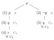
Example 7.29 (the platform, cont’d: the switches that follow). Harriet runs the search on the five rules of Example 7.14. No clause is a unit at the start, since each has at least two literals, so she decides $p$ , trying it on first. The root carries the clause set. Beside each other node is the rule that wrote it: d for a decision, and the clause for a forced move. A closed branch ends in a cross, with the clause it falsifies.

A DPLL tree drawn top down. Below the root S the tree forks by decision into node 1, p, and node 2, not p. Under p: node 3, q, forced by C1; node 4, r, forced by C4; then a cross, C5 falsified. Under not p: node 5, q, forced by C3; then a cross, C2 falsified.

In list form:

nodes 1 and 2 are the decision on $p$ ;
under ${p}$ , the clause $C_{1} = \neg p \lor q$ is a unit and forces $q$ (node 3); under ${p, q}$ , the clause $C_{4} = \neg p \lor \neg q \lor r$ is a unit and forces $r$ (node 4); and under ${p, q, r}$ the clause $C_{5} = \neg p \lor \neg q \lor \neg r$ is falsified;
under ${\neg p}$ , the clause $C_{3} = p \lor q$ forces $q$ (node 5), and under ${\neg p, q}$ the clause $C_{2} = \neg q \lor p$ is falsified.

Both branches close, so the tree is closed: five nodes, one decision and two dead branches, against the eight rows of the truth table.

Choosing the letter

The one choice the procedure leaves open is which letter to decide on, the branching heuristic, and much of the engineering of a solver lies in choosing well. Take the clause set

\neg p \lor q, \neg p \lor r, \neg p \lor s, p \lor t, p \lor \neg t .

Deciding $p$ first, and trying it on, forces $q$ , $r$ and $s$ by the first three clauses, and every clause is satisfied: one decision. Deciding $q$ , $r$ or $s$ first forces nothing, and a second decision is needed before the search ends. A common rule of thumb is to decide a letter that occurs in many short clauses, so that the decision forces as much as possible on both sides. Which side to try first is a choice too, and solvers make it by a second heuristic. Nothing in this chapter depends on the choice, since the results below hold for every order; what depends on it is the size of the tree.⁴

Correctness

Three things need checking: that the search stops, that a closed tree is never wrong, and that an unsatisfiable clause set always produces one.

Lemma 7.30 (termination). Let $S$ be a clause set with $n$ letters.

No branch of a DPLL tree for $S$ has more than $n$ nodes below the root.
There is a complete DPLL tree for $S$ .
$DPLL (S)$ stops.

Proof. One part at a time.

(i). A decide step and a unit step each add to a branch a literal whose letter the branch does not yet decide, and $S$ has only $n$ letters.
(ii). Start from the root, apply a step to a branch that is not complete, and repeat. A tree in which every node has at most two children and, by (i), every branch at most $n$ nodes below the root has fewer than $2^{n + 1}$ nodes, and each step adds a node, so this stops. When it stops the tree is complete: a branch that is neither closed nor finished has a clause that is neither satisfied nor falsified, and so a literal whose letter $u_{B}$ does not decide, and that letter can be decided.
(iii). Each step of PROPAGATE and each recursive call of SEARCH adds a literal on an undecided letter of $S$ , so each call makes at most $n$ steps of propagation and the recursion is at most $n$ deep.

□

Theorem 7.31 (soundness of DPLL). If a clause set $S$ is satisfiable, then no DPLL tree for $S$ is closed.

Proof. Let $v ⊨ S$ . Call a branch $B$ faithful to $v$ if $u_{B} ⪯ v$ . We show, by induction on the construction of the tree, that every DPLL tree for $S$ has a faithful branch.

Start. The root alone is faithful, since its partial valuation is $\emptyset$ , and $\emptyset ⪯ v$ .
Decide, on a faithful branch $B$ . The valuation $v$ makes $p$ true or false, so $u_{B} \cup {p} ⪯ v$ or $u_{B} \cup {\neg p} ⪯ v$ , and one of the two new branches is faithful.
Unit, on a faithful branch $B$ . The clause $C$ is a unit on $B$ with undecided literal $ℓ$ , and $v ⊨ C$ , so $v ⊨ ℓ$ by part (iii) of the lemma on the status of a clause. Hence $u_{B} \cup {ℓ} ⪯ v$ , and the branch with $ℓ$ added is faithful.
A step on another branch. It leaves the faithful branch as it was.

A faithful branch is open: if a clause were falsified on it, then by part (ii) of the lemma $v ⊭ C$ for that clause $C$ . So no DPLL tree for $S$ is closed. □

In words: a closed DPLL tree is a certificate that no valuation satisfies $S$ .

Proposition 7.32 (finished branches). Let $B$ be a finished branch of a DPLL tree for $S$ . Then $v ⊨ S$ for every valuation $v$ with $u_{B} ⪯ v$ .

Proof. The branch is finished, so $u_{B} ⊨ C$ for every $C \in S$ , and part (i) of the lemma on the status of a clause gives $v ⊨ C$ . □

Theorem 7.33 (completeness of DPLL). If a clause set $S$ is unsatisfiable, then every complete DPLL tree for $S$ is closed.

Proof. Suppose a complete DPLL tree for $S$ has an open branch $B$ . Being complete and open, $B$ is finished. By the proposition on finished branches, $v ⊨ S$ for every $v$ with $u_{B} ⪯ v$ , and there is such a $v$ : give every letter that $u_{B}$ does not decide the value $false$ . So $S$ is satisfiable. □

In words: when no valuation satisfies $S$ , every search carried to the end produces the certificate.

Theorem 7.34 (correctness of DPLL). For every clause set $S$ , the procedure $DPLL (S)$ stops, and

it returns CLOSED if and only if $S$ is unsatisfiable;
when it returns OPEN(u), $v ⊨ S$ for every valuation $v$ with $u ⪯ v$ .

Proof. It stops by termination, and it returns one of two answers.

It returns OPEN(u). Then $u ⊨ S$ , so $v ⊨ S$ for every $v$ with $u ⪯ v$ , by part (i) of the lemma on the status of a clause; in particular $S$ is satisfiable.
It returns CLOSED. The branches it built form a DPLL tree for $S$ , every one of them closed, so by soundness $S$ is unsatisfiable.

So it returns CLOSED exactly when $S$ is unsatisfiable. □

The proof did not use completeness, which says more: when $S$ is unsatisfiable, every search closes, however its choices go.

Remark 7.35 (looking back: the truth lemma). The proof of soundness followed a single valuation down the tree, and the proof of completeness read a valuation off a branch. That reading is the truth lemma of the completeness proof in Chapter 6, shrunk to one sentence.

Example 7.36 (the platform, cont’d: a setting). The colleague who wrote the rules looks at Harriet’s closed tree and says that the second rule is wrong: fast syncs fill the cache when there are any, but offline-mode does not need fast-sync. Harriet strikes out $C_{2}$ and runs the procedure on ${C_{1}, C_{3}, C_{4}, C_{5}}$ .

Nothing is forced, so the procedure decides $p$ . On the $p$ side, $C_{1}$ forces $q$ , $C_{4}$ forces $r$ , and $C_{5}$ is falsified. On the $\neg p$ side, $C_{3}$ forces $q$ , and $u = {\neg p, q}$ satisfies all four clauses: $C_{1}$ , $C_{4}$ and $C_{5}$ because $u ⊨ \neg p$ , and $C_{3}$ because $u ⊨ q$ . The procedure returns OPEN with $u$ : fast-sync off, offline-mode on, and compression as you please. Four lines check the four rules against that setting, and Harriet ships it.

Easy to check, hard to find

Both answers of the procedure come with evidence that anyone can check without trusting the solver. The answer OPEN(u) comes with $u$ , and checking it means finding, in each clause, a literal of $u$ : one bit per letter, and one reading of each clause. The answer CLOSED comes with the tree, and checking it means checking each node against the rules of Figure 7.2; that needs no cleverness, but it costs as much as the tree is big, and the tree can be exponential. For some clause sets it must be: the optional Section 7.8 shows that for the pigeonhole sets, which say that $n + 1$ pigeons do not fit into $n$ holes, every closed tree is exponential in $n$ . A search that does not know in advance which answer it will give may have to build most of such a tree before it can give either. The gap between checking an answer and finding one is not a fault of the method but the shape of the problem itself.

Deciding whether a clause set is satisfiable is the problem called sat, the first problem shown to be NP-complete.⁵ That means two things. Its “yes” answers can be checked quickly, by the certificate for OPEN. And every problem whose “yes” answers come with evidence that can be checked quickly can be turned, quickly, into an instance of sat, so a fast method for sat would be a fast method for all of them. (“Quickly” means in a number of steps bounded by a polynomial in the size of the input, such as its square or its cube.)

The problems whose “yes” answers can be checked quickly form the class NP, and those that can be decided quickly the class P. Whether a fast method for sat exists is the question whether $P = NP$ , and nobody knows.

What is known is that the problem is decided, by the procedure of this chapter; that the solvers built on it settle instances with millions of switches; and that no method is known to be fast on every instance, nor is one known to be impossible.

Remark 7.37 (SAT and SMT). Many questions about programs and hardware are about numbers, arrays and bit-strings, and an atomic formula such as $x + 1 > y$ is true or false according to the values of $x$ and $y$ , not by a switch of its own. An SMT solver, for satisfiability modulo theories, pushes such questions down to sat. It reads each atomic formula as a letter and runs DPLL; whenever the search has set some atomic formulas true and others false, it asks a decision procedure for the theory (arithmetic, arrays, equality between terms) whether that combination can hold together, and if it cannot, as with $x > 1$ and $x < 0$ both on, the reason is added as a new clause. The engine is the procedure of this section.

7.4 From Sentences to Clauses

The simpler problem is solved. A question $Γ ⊨ φ$ without quantifiers becomes a clause set, and DPLL decides whether some valuation satisfies it. Now for the problem we actually have. The constraints of a real question say “every” and “some”, and no setting of finitely many switches says either. The reduction of $Γ ⊨ φ$ , quantifiers and all, to sat problems takes three moves.

Put the quantifiers in one place. Each sentence is rewritten, without changing what it says, so that all its quantifiers stand in a row at the front.
Name the existentials. Each “some” is replaced by a name for its witness, a new function of the universal variables before it, as a search by hand names the someone it is looking for. Only universal quantifiers are left, and the sentence becomes a set of clauses with variables in them.
Instantiate the universals. The clauses are tested at the names, one instance at a time, and each instance is a clause over switches (Section 7.5). The instances go to DPLL level by level (Section 7.6).

The first two moves are routine rewriting, and this section treats them as a black box: it says what goes in, what comes out, and what is guaranteed. The optional Section 7.7 opens the box. The third move is where the work is, and it takes the next two sections. From here on the formulas are again the first-order formulas of Chapter 6, over a signature $Σ$ .

Remark 7.38 (a second route: SMT). There is a second way to bring a first-order question to a SAT solver. An SMT solver (Remark 7.37) keeps the quantifiers and deals with them on the side, adding instances of the universal sentences to its propositional problem as the search goes. The route of this chapter removes the quantifiers first, and then proves that instances are enough. The two routes meet in Section 7.6.

What comes out of the box is a set of clauses with variables in them, and the first thing to settle is what such a clause means.

Definition 7.39 (first-order clause). A first-order clause is built like a propositional clause, but its literals are atomic formulas about terms, and the terms may contain variables.

Formally, a clause over $Σ$ is a finite set of literals, that is, of atomic $Σ$ -formulas and their negations, possibly with variables, and a clause set is a finite set of clauses. A clause with no variables is a ground clause.

For instance, of the two clauses

\neg P (x) \lor Q (f (x)) and \neg P (c) \lor Q (f (c))

the second is ground.

Definition 7.40 (satisfying a first-order clause set). A structure satisfies a clause when the clause holds of everybody: whatever its variables stand for, one of its literals is true.

Formally, let $M$ be a $Σ$ -structure and $C$ a clause over $Σ$ . Then $M ⊨ C$ if

for every assignment s, M, s ⊨ ℓ for some ℓ \in C,

and $M ⊨ S$ , for a clause set $S$ , if $M ⊨ C$ for every $C \in S$ .

In words: a clause is read as the universal closure of the disjunction of its literals. For a clause $C = ℓ_{1} \lor \dots \lor ℓ_{n}$ with variables $x_{1}, \dots, x_{k}$ ,

M ⊨ C exactly when M ⊨ \forall x_{1} \dots \forall x_{k} (ℓ_{1} \lor \dots \lor ℓ_{n}) .

In particular, for a ground clause $C$ , $M ⊨ C$ exactly when $v_{M} ⊨ C$ in the sense of Section 7.2, where $v_{M}$ is the valuation that gives each atomic sentence its truth value in $M$ .

The box adds symbols to the signature. If $Σ^{+}$ is $Σ$ with some symbols added, a $Σ^{+}$ -structure $M = (D, I)$ has a restriction to $Σ$ ,

M ↾ Σ = (D, I ↾ Σ),

the same domain with the added symbols forgotten, as in the completeness proof of Chapter 6. A $Σ$ -sentence mentions none of the added symbols, so it is true in $M$ exactly when it is true in $M ↾ Σ$ .

Theorem 7.41 (the clause form). There is an algorithm that takes each finite set $Γ$ of $Σ$ -sentences to a clause set $cl (Γ)$ over a signature $Σ^{+}$ , which is $Σ$ with new function and constant symbols added, such that

$Γ$ is satisfiable if and only if $cl (Γ)$ is;
if $M ⊨ cl (Γ)$ , then $M ↾ Σ ⊨ Γ$ .

The clause set $cl (Γ)$ that the algorithm returns is called the clause form of $Γ$ . In words: the clause form keeps the verdict, (i), and the evidence comes back with it, (ii). It does not keep the meaning, since it speaks of symbols that $Γ$ does not have: $Γ$ and $cl (Γ)$ are equisatisfiable, not true in the same structures. The new symbols name the witnesses of the existential quantifiers, and are called Skolem functions and Skolem constants. For instance, “everyone has someone who earns more”, $\forall x \exists y Richer (y, x)$ , becomes the single clause

Richer (f (x), x),

with $f (x)$ naming whoever earns more than $x$ , over $Σ^{+} = Σ \cup {f}$ ; and “someone earns more than everyone”, $\exists y \forall x Richer (y, x)$ , becomes $Richer (a, x)$ over $Σ \cup {a}$ , with the constant $a$ naming that someone. The optional Section 7.7 gives the algorithm and the proof; for the problem sheets and the rest of the chapter, the theorem is all that is needed.

Example 7.42 (the company, cont’d: the policy as clauses). To decide whether ${P_{1}, P_{2}} ⊨ C$ , Harriet needs the clause form of ${P_{1}, P_{2}, \neg C}$ , a set of sentences over the company signature $Σ$ . The two rules have no existential quantifier, and $\neg C$ says that some engineer reports to an engineer; its witness gets the Skolem constant $a$ , the name her first search in Example 7.4 gave it. So $Σ^{+} = Σ \cup {a}$ , and the clause form is four clauses:

\begin{aligned} C_{1} & = \neg Eng (x) \lor Mgr (boss (x)) & an engineer’s boss is a manager; \\ C_{2} & = \neg Mgr (x) \lor \neg Eng (x) & no manager is an engineer; \\ C_{3} & = Eng (a) & a is an engineer; \\ C_{4} & = Eng (boss (a)) & so is a ’s boss. \end{aligned}

By the reduction lemma and the theorem on the clause form,

{P_{1}, P_{2}} ⊨ C if and only if {C_{1}, C_{2}, C_{3}, C_{4}} is unsatisfiable .

The colleague’s weaker policy is ${C_{1}, C_{3}, C_{4}}$ , which is satisfiable: the two-person company $M$ of Example 7.4, with $a$ naming the engineer who reports to an engineer, has $M ⊨ {C_{1}, C_{3}, C_{4}}$ , and $M ↾ Σ$ is the counter-model of that example.

Remark 7.43 (equality). The symbol $=$ is a relation symbol like any other, and in a clause set it is treated as one: nothing in the definitions above knows that it means identity. A set of sentences that is to reason about identity must say what identity is, by the equality axioms, which Definition 6.36 states for any signature, and so must a clause set. Those axioms are infinitely many, one for every formula; for a clause set over a finite signature, finitely many clauses do the same work, and we call them the equality clauses. They are reflexivity, symmetry, transitivity, and one congruence clause for each argument place of each function symbol and of each relation symbol other than $=$ , saying that equals may be put for equals in that place. For $=$ itself no congruence clause is needed: symmetry and transitivity already do the work. For a signature with a one-place function symbol $f$ , one-place relation symbols $P$ and $Q$ , and a two-place relation symbol $R$ besides $=$ , the congruence clauses are

\begin{matrix} \neg (x = y) \lor f (x) = f (y), \\ \neg (x = y) \lor \neg P (x) \lor P (y), \neg (x = y) \lor \neg Q (x) \lor Q (y), \\ \neg (x = y) \lor \neg R (x, z) \lor R (y, z), \\ \neg (x = y) \lor \neg R (z, x) \lor R (z, y) . \end{matrix}

Exercise 7.10 writes out the rest and puts a question about identity through the machinery of this chapter. A structure that satisfies such a clause set interprets $=$ as some relation that behaves like identity but need not be it. A remark in the next section shows how to recover from it a structure in which $=$ is identity.

7.5 Herbrand’s Theorem

Two moves of the reduction are made: the question $Γ ⊨ φ$ has become whether a set of clauses with variables in them, all universal, is unsatisfiable. What is left is the third move, the universals. A clause with a variable speaks of every element of every structure (five people, the natural numbers, the real line), and a solver cannot look at every structure. It need not. A search by hand looks only at the things it can name, starting from the names it has, and this section proves that it is right to, in two steps.

If a clause set is satisfied by any structure at all, it is satisfied by one made of names, and such a structure is a setting of the switches, one for each atomic sentence about the names.
If it has no model, finitely many of its instances at those names already show it.

The names are built from the symbols of the clauses. A clause set comes over some signature, and that signature may have symbols the clauses never use (the clauses of Example 7.42 mention neither $ceo$ nor $Richer$ ). A search should name things only through the symbols its clauses use, so this section works over the signature of the clauses themselves. Nothing is lost by doing so. Symbols that a clause set does not mention make no difference to whether it is satisfiable: a structure for the larger signature can be restricted to the smaller one, and a structure for the smaller one can be expanded by giving the other symbols any meaning.

Definition 7.44 (the signature of a clause set). The signature of a clause set is the vocabulary it actually uses.

Formally, the signature $Σ_{S}$ of a clause set $S$ consists of the constant, function and relation symbols that occur in $S$ , with one new constant symbol added if no constant occurs in $S$ .

The extra constant is there because a signature with no constant names nothing, and a set of names that is to serve as the domain of a structure must not be empty. A structure $M$ for a larger signature satisfies $S$ exactly when its restriction $M ↾ Σ_{S}$ does, the added constant, if any, being given some element to name.

Definition 7.45 (Herbrand universe). The Herbrand universe of a clause set is the set of everything the clause set can name.

Formally, the Herbrand universe $H (S)$ of a clause set $S$ is the set of closed $Σ_{S}$ -terms.

In words: start from the constants and apply the function symbols in every possible way. For a clause set whose only constant is $c$ and whose only function symbol is a one-place $f$ , the universe is $c$ , $f (c)$ , $f (f (c))$ , and so on.

Definition 7.46 (level). The level of a closed term is the depth to which function symbols are nested in it.

Formally, the level of a closed term $t$ is defined by recursion on the shape of $t$ :

level (t) : = {\begin{cases} 0 & if t is a constant, \\ 1 + max_{i} level (t_{i}) & if t is f (t_{1}, \dots, t_{n}) . \end{cases}

For a clause set $S$ and $k \geq 0$ , we write $H_{k} (S)$ for the set of terms of $H (S)$ of level at most $k$ .

For instance, $f (f (c))$ has level $2$ , and in the universe above $H_{1} = {c, f (c)}$ .

The universe grows level by level, and it is worth seeing how fast. Figure 7.3 draws it for a clause set with a constant $c$ and two one-place function symbols $f$ and $g$ . Each level holds twice as many terms as the level below, so the picture is a pyramid standing on its point, and $H_{k} (S)$ is everything from the point up to level $k$ . Every $H_{k} (S)$ is finite, and each contains the one before:

H_{0} (S) \subseteq H_{1} (S) \subseteq H_{2} (S) \subseteq \dots,

and together they make up the whole universe, which is infinite. A search that works through the universe must therefore do so one level at a time, and that is how the first-order procedure of Section 7.6 works through it.

Figure 7.3. The Herbrand universe, level by level.

Definition 7.47 (Herbrand base). The Herbrand base of a clause set is the set of atomic sentences it can form about its names: the switches of a first-order search.

Formally, the Herbrand base of a clause set $S$ is the set of atomic $Σ_{S}$ -sentences $R (t_{1}, \dots, t_{n})$ , with $R$ an $n$ -place relation symbol of $Σ_{S}$ and $t_{1}, \dots, t_{n} \in H (S)$ .

For instance, if $Σ_{S}$ above has one relation symbol, a one-place $P$ , the base is $P (c)$ , $P (f (c))$ , $P (f (f (c)))$ , and so on.

Definition 7.48 (Herbrand structure, Herbrand model). A Herbrand structure is a structure whose elements are names, each naming itself.

Formally, let $S$ be a clause set. A Herbrand structure for $S$ is a $Σ_{S}$ -structure $H = (H (S), I)$ in which

$I (c) = c$ for each constant symbol $c$ ;
$I (f) (t_{1}, \dots, t_{n}) = f (t_{1}, \dots, t_{n})$ for each $n$ -place function symbol $f$ ;
$I (R)$ is any set of $n$ -tuples of closed terms, for each $n$ -place relation symbol $R$ .

A Herbrand model of $S$ is a Herbrand structure $H$ for $S$ that is a model of $S$ , that is, with $H ⊨ S$ .

In words: the domain is the names, the constants and function symbols do nothing but build names, and all the freedom is in the relations. A Herbrand structure is therefore nothing more than a choice of true or false for each atomic sentence of the base; that is, a Herbrand structure is a valuation of the Herbrand base: a setting of the switches, one switch for each atomic sentence about the names. A search for a Herbrand model is therefore a search for a setting.

Remark 7.49 (looking back: the term structure). The completeness proof of Chapter 6 built its structure out of closed terms, each naming itself, with the relations chosen by a maximal consistent set. That structure was a Herbrand structure, for the signature with the witnesses added, and the truth lemma said that it satisfied the set. Nothing in this section is new in kind; what is new is that the relations are now chosen by a search rather than by a construction that lists every sentence.

Example 7.50 (the company, cont’d: the names of the policy). The clause set $S = {C_{1}, C_{2}, C_{3}, C_{4}}$ of Example 7.42 is over $Σ^{+}$ , the company signature with $a$ added, but it uses only four of its symbols: $Σ_{S}$ has the constant $a$ , the function symbol $boss$ and the relation symbols $Eng$ and $Mgr$ , and no $ceo$ or $Richer$ . Its Herbrand universe is

a, boss (a), boss (boss (a)), boss (boss (boss (a))), \dots,

one term for each level: $H_{0} = {a}$ , $H_{1} = {a, boss (a)}$ , and so on. It is infinite, because $boss$ can be applied again to its own result, and in a Herbrand structure the chain of bosses never comes back on itself. The base is the atomic sentences $Eng (t)$ and $Mgr (t)$ for $t$ in the universe. If a Herbrand structure $H$ makes every $Eng (t)$ and every $Mgr (t)$ true, for instance, then $H ⊨ {C_{1}, C_{3}, C_{4}}$ and $H ⊭ C_{2}$ .

Instances

To say what a clause demands of a Herbrand structure, we put names in for its variables, several variables at once. The tool for that is a substitution.

Definition 7.51 (substitution). A substitution is a finite list of instructions, each saying which term to put in for one variable.

Formally, a substitution is a finite list $σ = [t_{1} / x_{1}, \dots, t_{n} / x_{n}]$ of pairs, each of a term $t_{i}$ and a variable $x_{i}$ , in which the variables $x_{1}, \dots, x_{n}$ are distinct. We also write it $[\bar{t} / \bar{x}]$ .

For instance, $[boss (y) / x, ceo / z]$ says: put $boss (y)$ for $x$ and $ceo$ for $z$ . It says nothing about $y$ , which it leaves alone. The empty list $[]$ is a substitution too, and changes nothing.

Substitutions are applied to terms, atomic formulas, literals and clauses, which for short we call expressions.

Definition 7.52 (applying a substitution). Applying a substitution to an expression puts the terms in for the variables, everywhere and all at once.

Formally, let $σ = [t_{1} / x_{1}, \dots, t_{n} / x_{n}]$ be a substitution. For an expression $e$ , the expression $e σ$ is defined by recursion on the shape of $e$ :

e σ : = {\begin{cases} t_{i} & if e is the variable x_{i}, \\ y & if e is a variable y other than x_{1}, \dots, x_{n}, \\ f (u_{1} σ, \dots, u_{m} σ) & if e is f (u_{1}, \dots, u_{m}), \\ R (u_{1} σ, \dots, u_{m} σ) & if e is R (u_{1}, \dots, u_{m}), \\ \neg (A σ) & if e is \neg A, with A atomic, \\ {ℓ_{1} σ, \dots, ℓ_{m} σ} & if e is the clause {ℓ_{1}, \dots, ℓ_{m}} . \end{cases}

In the third line $f$ may be a constant, with $m = 0$ , and then $e σ$ is $e$ . In words: every occurrence of each $x_{i}$ is replaced by $t_{i}$ , and the terms put in are not looked at again. That is what “all at once” means: $Richer (x, y) [y / x, x / y]$ is $Richer (y, x)$ , whereas putting $y$ for $x$ and then $x$ for $y$ , one after the other, would give $Richer (x, x)$ . An expression has no quantifiers, so nothing in it can capture a variable, and no renaming is ever needed.

Remark 7.53 (looking back: substitution for one variable). For one variable, $e [t / x]$ is the substitution $φ [t / x]$ of Chapter 6, restricted to formulas without quantifiers. Its side conditions, which stop a quantifier of $φ$ from capturing a variable of $t$ , never arise here.

Definition 7.54 (instance, ground instance). An instance of a clause is what the clause says about particular terms, and a ground instance is what it says about particular names.

Formally, let $C$ be a clause. An instance of $C$ is a clause $C σ$ , for a substitution $σ$ . If $C$ is a clause of a clause set $S$ , with variables $x_{1}, \dots, x_{n}$ , a ground instance of $C$ is a clause $C [t_{1} / x_{1}, \dots, t_{n} / x_{n}]$ with $t_{1}, \dots, t_{n} \in H (S)$ .

For instance, the clause $\neg P (x) \lor Q (f (x), y)$ has the instance $\neg P (f (z)) \lor Q (f (f (z)), y)$ , by $[f (z) / x]$ ; in a clause set with the constant $c$ it has the ground instance $\neg P (c) \lor Q (f (c), c)$ , by $[c / x, c / y]$ . A ground instance is a ground clause, since every variable of $C$ has been given a closed term.

Definition 7.55 (the ground instances of a clause set). The ground instances of a clause set are everything its clauses say about its names, and those at level $k$ use only names of level at most $k$ .

Formally, let $S$ be a clause set. We write $Gr (S)$ for the set of all ground instances of all clauses of $S$ , and, for $k \geq 0$ , ${Gr}_{k} (S)$ for the set of those ground instances $C [t_{1} / x_{1}, \dots, t_{n} / x_{n}]$ , with $C \in S$ and $x_{1}, \dots, x_{n}$ its variables, in which $t_{1}, \dots, t_{n} \in H_{k} (S)$ .

Each ${Gr}_{k} (S)$ is a finite clause set over the Herbrand base, and $Gr (S)$ is their union, infinite as soon as the universe is and some clause has a variable.

Example 7.56 (the company, cont’d: the ground instances of the policy). For the four clauses of Example 7.42, ${Gr}_{0}$ has four clauses, the two rules instantiated at $a$ and the two units; ${Gr}_{1}$ has six:

\begin{aligned} \neg Eng (a) \lor Mgr (boss (a)), & \neg Eng (boss (a)) \lor Mgr (boss (boss (a))), \\ \neg Mgr (a) \lor \neg Eng (a), & \neg Mgr (boss (a)) \lor \neg Eng (boss (a)), \\ Eng (a), & Eng (boss (a)) . \end{aligned}

Lemma 7.57 (a Herbrand structure is a valuation). For a Herbrand structure $H$ for $S$ , write $v_{H}$ for the valuation of the Herbrand base that makes an atomic sentence true exactly when it is true in $H$ . Then

H ⊨ S if and only if v_{H} ⊨ Gr (S) .

Proof. First, every closed term $t$ names itself, $Val (t) = t$ : by induction on $t$ , a constant names itself by the first item of the definition of a Herbrand structure, and $f (t_{1}, \dots, t_{n})$ names $I (f) (t_{1}, \dots, t_{n}) = f (t_{1}, \dots, t_{n})$ by the second and the induction hypothesis.

Now let $C$ be a clause of $S$ with variables $\bar{x}$ . An assignment $s$ into $H$ gives each $x_{i}$ a closed term $s (x_{i})$ , which names itself; so, by the substitution lemma, a literal of $C$ is true under $s$ exactly when the literal of $C [s (\bar{x}) / \bar{x}]$ is true in $H$ outright. Every ground instance of $C$ is $C [s (\bar{x}) / \bar{x}]$ for some assignment $s$ , the one that sends each $x_{i}$ to the term put in for it, so $H ⊨ C$ exactly when every ground instance of $C$ has a literal true in $H$ . A ground literal is true in $H$ exactly when $v_{H}$ makes it true, by the atomic clause of the definition of satisfaction and the definition of $v_{H}$ ; so $H ⊨ C$ exactly when $v_{H} ⊨ C^{'}$ for every ground instance $C^{'}$ of $C$ . □

In words: to say what a Herbrand structure does to a clause set is to run through the ground instances, and that is a propositional matter.

Lemma 7.58 (Herbrand models suffice). A clause set is satisfiable if and only if it has a Herbrand model.

Proof. A Herbrand model is a model, so only the forward direction needs an argument. Let $M ⊨ S$ , where by the paragraph after the definition of $Σ_{S}$ we may take $M$ to be a $Σ_{S}$ -structure, and let $H$ be the Herbrand structure in which an atomic sentence $R (t_{1}, \dots, t_{n})$ of the base is true exactly when it is true in $M$ . By the lemma it is enough to show that $v_{H} ⊨ C [\bar{t} / \bar{x}]$ for every ground instance of every clause $C$ of $S$ .

Since $M ⊨ C$ , some literal of $C$ is true in $M$ under the assignment $s$ that sends each $x_{i}$ to the element $Val (t_{i})$ of $M$ ; by the substitution lemma, that literal with $\bar{t}$ put in is true in $M$ outright. It is a literal of $C [\bar{t} / \bar{x}]$ , a ground literal, and by the definition of $H$ it is true in $H$ , that is, $v_{H}$ makes it true. So $v_{H} ⊨ C [\bar{t} / \bar{x}]$ , hence $H ⊨ S$ , and $H$ is a Herbrand model of $S$ . □

In words: given a structure that satisfies the clause set, read off which atomic sentences it makes true and forget everything else; what is left is a structure made of names that satisfies it too. The proof is short because it uses only the quantifier clauses of the definition of satisfaction, the substitution lemma, and the fact that in a structure made of names every element has one.

So a search for a counter-model may confine itself to the things it can name: if a counter-model exists at all, one exists that is made of names. One more step turns “among those” into “among finitely many of those”, and it needs a consequence of the completeness of $NK$ that has not yet been named.

Lemma 7.59 (compactness). Let $Γ$ be a set of sentences over a countable signature. If every finite subset of $Γ$ has a model, then $Γ$ has a model.

Proof. We prove the contrapositive: if $Γ$ has no model, some finite subset has none. Suppose $Γ$ has no model. Then $Γ ⊨ ⊥$ , since there is no model of $Γ$ in which $⊥$ fails, and by the completeness of $NK$ there is a derivation of $⊥$ from $Γ$ . A derivation is a finite tree, so it has finitely many open hypotheses, which form a finite subset $Δ$ of $Γ$ with $Δ ⊢_{NK} ⊥$ . By soundness $Δ ⊨ ⊥$ , so $Δ$ has no model. □

In words: an infinite set of demands can only fail for a finite reason, and the reason is that proofs are finite.

Theorem 7.60 (Herbrand’s theorem). For every clause set $S$ , the following are equivalent:

there is no structure $M$ with $M ⊨ S$ ;
there is a finite $Δ \subseteq Gr (S)$ with no valuation $v ⊨ Δ$ , reading $Δ$ as a propositional clause set over the Herbrand base;
there is a $k$ with no valuation $v ⊨ {Gr}_{k} (S)$ .

Proof. One implication at a time.

(ii) implies (i). Suppose $M ⊨ S$ . By the lemma that Herbrand models suffice there is a Herbrand structure $H ⊨ S$ , and by the lemma before it $v_{H} ⊨ Gr (S)$ , so $v_{H} ⊨ Δ$ for every $Δ \subseteq Gr (S)$ .
(i) implies (ii). The ground clauses of $Gr (S)$ , each read as the disjunction of its literals, are sentences over a finite, hence countable, signature, and no structure satisfies them all: the truth values of the ground atomic sentences in such a structure would give a valuation $v ⊨ Gr (S)$ , hence a Herbrand model of $S$ by the lemma that a Herbrand structure is a valuation. By compactness some finite $Δ \subseteq Gr (S)$ has no model, and by the same argument no valuation $v ⊨ Δ$ .
(ii) and (iii) are equivalent. A finite $Δ \subseteq Gr (S)$ uses finitely many closed terms, and if $k$ is the largest of their levels, $Δ \subseteq {Gr}_{k} (S)$ ; a valuation that satisfies ${Gr}_{k} (S)$ satisfies $Δ$ . And ${Gr}_{k} (S)$ is itself a finite subset of $Gr (S)$ .

□

In words: a set of constraints about everybody has no model exactly when finitely many of its instances, at finitely many names, already clash.

Example 7.61 (the company, cont’d: six clauses). No valuation satisfies ${Gr}_{1}$ , the six clauses of Example 7.56, and unit propagation alone shows it. The unit $Eng (a)$ must be true, so by the first clause $Mgr (boss (a))$ must be; the unit $Eng (boss (a))$ must be true; and now the clause $\neg Mgr (boss (a)) \lor \neg Eng (boss (a))$ has both its literals false. These are the lines of Harriet’s first search, one for one: $a$ is an engineer, so her boss is a manager, so her boss is not an engineer, but her boss is. By Herbrand’s theorem ${C_{1}, \dots, C_{4}}$ is unsatisfiable, so by the reduction lemma and the theorem on the clause form, ${P_{1}, P_{2}} ⊨ C$ .

The four clauses of ${Gr}_{0}$ do not suffice: the valuation that makes $Eng (a)$ , $Eng (boss (a))$ and $Mgr (boss (a))$ true and $Mgr (a)$ false satisfies them. The clash needs the second rule at $boss (a)$ , one level up, which is the line of her search that applied $P_{2}$ to $a$ ’s boss.

What the theorem does not say

Herbrand’s theorem gives no bound on the level at which the clash appears, and the level needed can be large. Nor does it say anything when no clash appears. If ${Gr}_{0}, {Gr}_{1}, \dots, {Gr}_{100}$ are each satisfiable, the theorem does not say that $S$ is, and it cannot: for ${P (c), \neg P (x) \lor P (f (x))}$ every ${Gr}_{k}$ is satisfiable, and so is the set; for another set, every ${Gr}_{k}$ up to some large $k$ may be satisfiable and the next one not. For a satisfiable set the evidence has to be a structure that satisfies it, and a valuation that satisfies the instances ${Gr}_{k} (S)$ of a single level is not one: it is a choice of truth values for the atomic sentences that occur in ${Gr}_{k} (S)$ , and says nothing about the instances above. Can any finite amount of work ever certify that a clause set is satisfiable? This chapter raises the question and does not settle it.

Remark 7.62 (equality in a Herbrand structure). When $=$ is among the symbols and the equality clauses of Remark 7.43 are in $S$ , a Herbrand structure that satisfies $S$ interprets $=$ as some relation $E$ on the closed terms that is reflexive, symmetric, transitive and respected by every symbol, which is all the clauses say. But $E$ need not be identity: $f (c) = c$ may hold in it while $f (c)$ and $c$ are different terms. To obtain a structure in which $=$ is identity, identify the terms that $E$ relates: the elements are the classes of terms, and the congruence clauses are exactly what makes the functions and relations well defined on the classes. The completeness proof of Chapter 6 makes the same move, for the same reason.

7.6 A Procedure for First-Order Logic

All three moves are made, and what is left is to run them. DPLL decides one finite clause set, and a first-order clause set has infinitely many ground instances. By Herbrand’s theorem, a clause set $S$ with variables is unsatisfiable exactly when some ${Gr}_{k} (S)$ is, and ${Gr}_{k} (S)$ is a finite clause set over finitely many letters, the atomic sentences that occur in it: just what DPLL decides. So:

procedure REFUTE(S)                   -- S a clause set, possibly with variables
    k := 0
    loop:
        if DPLL(GROUND(S, k)) = CLOSED: return UNSAT   -- the instances at level k
        k := k + 1

The procedure has no other exit, and that is not an oversight.

Theorem 7.63 (the first-order procedure). For every clause set $S$ , the call $REFUTE (S)$

returns UNSAT if $S$ is unsatisfiable;
runs for ever if $S$ is satisfiable.

Proof. If $S$ is unsatisfiable, some ${Gr}_{k} (S)$ is unsatisfiable by Herbrand’s theorem, and by the correctness of DPLL the call $DPLL ({Gr}_{k} (S))$ returns CLOSED at the latest at that $k$ , each earlier call having stopped by termination. If $S$ is satisfiable, some Herbrand structure $H$ satisfies it, and $v_{H}$ satisfies every ${Gr}_{k} (S)$ , so by soundness no call returns CLOSED and REFUTE never stops. □

In words: the procedure is a complete method for “no”, and no method at all for “yes”. Procedures of this kind have a name.

Definition 7.64 (semi-decision procedure). A semi-decision procedure for a property answers “yes” on every input that has the property, and never on one that lacks it.

Formally, let $A$ be a set of inputs. A procedure is a semi-decision procedure for $A$ if, for every input $x$ , it stops and answers that $x$ is in $A$ when $x \in A$ , and never gives that answer when $x \notin A$ .

So REFUTE is a semi-decision procedure for the set of unsatisfiable clause sets. For first-order logic, by the reduction lemma and the clause form of a set, that is a way of certifying in finite time every entailment that holds from finitely many premisses, and nothing for one that fails.

Example 7.65 (the company, cont’d: the policy, by machine). Harriet gives the four clauses of Example 7.42 to REFUTE. At level $0$ the four ground clauses of Example 7.61 go to DPLL, which propagates $Eng (a)$ , $Eng (boss (a))$ , $Mgr (boss (a))$ and $\neg Mgr (a)$ , finds every clause satisfied, and returns OPEN. At level $1$ the six ground clauses go to DPLL, which propagates $Eng (a)$ , $Eng (boss (a))$ and $Mgr (boss (a))$ , finds $\neg Mgr (boss (a)) \lor \neg Eng (boss (a))$ falsified, and returns CLOSED without a decision. The loop returns UNSAT: the rules entail the claim, by a single branch with no guess, like Harriet’s first search.

With the weaker policy ${C_{1}, C_{3}, C_{4}}$ the loop never returns. Figure 7.4 sets out both runs level by level. At levels $0$ and $1$ forced moves alone satisfy the ground clauses. At level $2$ there are five clauses and a decision, since $Mgr (boss (boss (a)))$ is forced but nothing decides $Eng (boss (boss (a)))$ ; and so on. Each level returns OPEN with a partial valuation that makes every $Eng (t)$ and $Mgr (t)$ it mentions true: the Herbrand structure in which everybody is an engineer and a manager, seen one level at a time. Harriet knows, from Example 7.4, that the weaker policy has a two-person counter-model. The procedure does not, and will not find out.

Policy	Level	Ground clauses	Decisions	Verdict
${C_{1}, C_{2}, C_{3}, C_{4}}$	$0$	$4$	$0$	`OPEN`
	$1$	$6$	$0$	`CLOSED`, so `UNSAT`
${C_{1}, C_{3}, C_{4}}$	$0$	$3$	$0$	`OPEN`
	$1$	$4$	$0$	`OPEN`
	$2$	$5$	$1$	`OPEN`
	…			`OPEN`, for ever

Figure 7.4. The policy by machine, level by level.

When $DPLL ({Gr}_{k} (S))$ returns OPEN, it has found a setting of the atomic sentences that occur in the instances at level $k$ , one that obeys those instances. That valuation satisfies ${Gr}_{k} (S)$ and nothing more. It does not satisfy $S$ , whose instances at level $k + 1$ the search has not seen (in Example 7.61 the instances at level $0$ are satisfiable, and the clash comes one level up). The verdict OPEN at a level is not a verdict about $S$ , and REFUTE rightly ignores it. Here the question raised after Herbrand’s theorem returns: can any finite amount of work certify that a clause set is satisfiable? For this procedure the answer is no: no finite level of the instances certifies satisfiability, and the loop does not try to. Whether a cleverer procedure could is the question of Chapter 8.

Choosing the instances

The loop lists every instance at a level, and most of what it lists is useless. A clash between instances of two clauses needs an atomic sentence that one instance contains and the other contains negated. Before anything is listed, the two clauses carry literals such as

Mgr (boss (x)) and \neg Mgr (y),

and the instances that can clash on them are those in which the two atomic formulas become the same, here by putting $boss (x)$ for $y$ . Finding such a substitution means solving an equation between them, written with $≐$ to keep it apart from the relation symbol $=$ ,

Mgr (boss (x)) ≐ Mgr (y),

and that can be done by machine. A short procedure, unification, either finds the most general solution, of which every other solution is an instance, or shows that there is none; and then the two literals never clash, at any level. Adding the instances that unification picks out before grounding never changes the verdict of the loop and never costs a level, and it often lets the loop close much sooner. The optional Section 7.8 gives the procedure and proves these claims.

Looking for small structures

There is a second search, the one everybody runs by hand when looking for a small counter-model: use as few elements as possible, start with one, and give every symbol the laziest meaning that works. It too is a propositional search. “Is $S$ satisfied by a structure with exactly $n$ elements?” becomes a clause set in three steps.

Name the elements $1, \dots, n$ , and take a letter for each atomic sentence over the names and for each equation $f (\bar{ı}) = j$ , with clauses saying that each $f (\bar{ı})$ has exactly one value.
Instantiate every clause of $S$ at every choice of names, replacing each term $f (\bar{ı})$ by a name $j$ and adding the literal $\neg (f (\bar{ı}) = j)$ .
Run DPLL: a setting that comes back is an $n$ -element structure that satisfies $S$ , and CLOSED says that none exists.

For instance, with $n = 2$ , step 2 turns the clause $\neg P (x) \lor Q (f (x))$ at $x = 1$ into two clauses, one for each value $f (1)$ may take:

\neg P (1) \lor \neg (f (1) = 1) \lor Q (1) and \neg P (1) \lor \neg (f (1) = 2) \lor Q (2),

that is, if $1$ is in $P$ and $f (1)$ is $j$ , then $j$ is in $Q$ ; and the same again at $x = 2$ . Run this for $n = 1, 2, 3, \dots$ alongside REFUTE, and one of the two answers whenever $S$ is unsatisfiable or satisfied by a finite structure. Exercise 7.9 carries the encoding out.

Example 7.66 (the company, cont’d: a company of one). For the weaker policy the search for small structures answers already at $n = 1$ : a company of one, an engineer and manager who is her own boss, obeys $C_{1}$ , $C_{3}$ and $C_{4}$ . So the two-person company of Example 7.4 was not the smallest counter-model.

Remark 7.67 (at work: SMT solvers and quantifiers). SMT solvers handle universal quantifiers much as the loop does when it chooses its instances. They keep a ground problem for their SAT engine, and from time to time add to it instances of the universal sentences. They choose the instances by heuristics rather than level by level. One adds an instance when the terms it needs turn up in the ground problem; another looks at the setting found so far, finds a universal sentence it breaks, and adds the instance that shows where. Like REFUTE, they may run for ever, and when they stop without a refutation they may answer “unknown” rather than produce a model.

A search that may not stop

A million switches is still a finite list, and that is the only reason every DPLL run stops: each branch ends when the switches run out, and once a question is cast as a finite clause set it is decided, however long the deciding takes. The first-order procedure has no such bound. It stops when the instances clash and only then, and whether they ever will is exactly the question being asked. A cleverer order of instances would not help: on some questions no instances ever clash, whatever the order, although a small counter-model exists. The clause set ${R (f (x), x), \neg R (y, g (y))}$ is one. A ground instance of the first clause has the shape $R (f (t), t)$ and one of the second the shape $\neg R (t^{'}, g (t^{'}))$ , so a clash needs $f (t)$ to be $t^{'}$ and $t$ to be $g (t^{'})$ , that is, $t$ to be $g (f (t))$ , which no term is. Yet the structure with two elements, each $R$ -related to the other, with $f$ sending each to the other and $g$ sending each to itself, satisfies the set, and the search for small structures, run alongside, finds it at $n = 2$ .

Worse, some satisfiable sets are satisfied only by infinite structures. The sentences $\forall x \exists y R (y, x)$ , $\forall x \neg R (x, x)$ and $\forall x \forall y \forall z (R (x, y) \land R (y, z) \to R (x, z))$ are satisfied by the natural numbers with $>$ for $R$ , and by no finite structure, since a finite chain of ever-greater elements must come back on itself and break the second sentence or the third. On such a set the loop never stops, the search for small structures never stops, and both are right not to (Examples 7.68 and 7.69 read both questions in the company).

Example 7.68 (the company, cont’d: a question that never closes). Does “everyone has someone who earns more than them” entail “someone earns more than everyone”? The clause form of the question is $Richer (f (x), x)$ together with $\neg Richer (y, g (y))$ , the second from the negated claim, $\forall y \exists x \neg Richer (y, x)$ : the clause set above, with $Richer$ for $R$ . So the loop runs for ever, and choosing the instances by unification adds nothing, since the two atomic formulas never unify. Yet a company of two in which each earns more than the other is a counter-model, which the search for small structures finds at $n = 2$ , once $n = 1$ has closed.

Example 7.69 (the company, cont’d: only infinite companies). The three constraints “everyone has someone who earns more”, “nobody earns more than themselves” and “if $x$ earns more than $y$ and $y$ more than $z$ then $x$ more than $z$ ” are the three sentences above, with $Richer$ for $R$ . No finite company obeys them all, and on them neither search ever stops.

The first-order procedure is a semi-decision procedure, then, and this chapter cannot say whether that is the best that can be done. The chapter’s own improvements were found by looking at where a method wasted its work, and each was real. A reader who has watched the loop run for ever on a question with a two-person answer will suspect that a cleverer search would stop. Chapter 8 is about that suspicion. What this chapter can say is where the cost sits: the Herbrand universe grows at least exponentially with the level as soon as there are two function symbols, or one with two places; equality multiplies the instances further; unification tames the second and nothing tames the first.

7.7 Prenex and Skolem Form (optional)

This section and the next are optional: the main line uses some of the results proved in them, but none of the proofs. This one opens the box of Section 7.4: it gives the algorithm behind the theorem on the clause form, and proves the theorem.

What makes a quantifier awkward? A search by hand applies each constraint to the things it has named, and a constraint of the form “for every $x$ , …” is ready for that: put a name in for $x$ and read what results. A constraint with “some” in it is not. “Some $x$ is …” does not say which, and the search has to invent a name for the someone before it can go on. Nor is a constraint ready when its quantifiers are buried inside it, under an arrow or a negation. There it is not even clear whether a quantifier says “every” or “some”: in

\neg \forall x Eng (x),

the $\forall$ says that someone is not an engineer.

The section deals with the second difficulty first, and then with the first. Here $\neg$ is a connective in its own right, as in Section 7.2, and $⊤$ abbreviates $\neg ⊥$ .

Negations first

As in Section 7.4, a literal is an atomic formula or the negation of one, and a formula is in negation normal form if it is built from literals, $⊥$ and $⊤$ by $\land$ , $\lor$ , $\forall$ and $\exists$ alone. The translation $nnf$ of Section 7.2 gets four more equations, two for the quantifiers and two for a negation in front of one:

\begin{aligned} nnf (\forall x ψ) & : = \forall x nnf (ψ), & nnf (\neg \forall x ψ) & : = \exists x nnf (\neg ψ), \\ nnf (\exists x ψ) & : = \exists x nnf (ψ), & nnf (\neg \exists x ψ) & : = \forall x nnf (\neg ψ) . \end{aligned}

In words: the negation of “everyone is …” is “someone is not …”, and the negation of “someone is …” is “nobody is …”. These are De Morgan’s laws for the quantifiers. The first equation of the definition now leaves every literal alone, atomic formulas and their negations included.

The lemma that negation normal form is faithful gains four cases. The two of substance are the quantifier clauses of the definition of satisfaction, read against the new equations. Take the equation for $\neg \exists x ψ$ , and let $M$ be a structure and $s$ an assignment. The induction hypothesis holds under every assignment, so under each $s [d / x]$ , and

\begin{aligned} M, s ⊨ \forall x nnf (\neg ψ) & ⟺ M, s [d / x] ⊨ nnf (\neg ψ) for every d \\ ⟺ M, s [d / x] ⊭ ψ for every d \\ ⟺ M, s ⊭ \exists x ψ \\ ⟺ M, s ⊨ \neg \exists x ψ, \end{aligned}

by the clause for $\forall$ , the induction hypothesis, the clause for $\exists$ and the clause for $\neg$ , in turn. The equation for $\neg \forall x ψ$ is the same with the quantifiers exchanged, and the two equations without a negation pass the claim straight down. So $nnf (φ)$ is true in a structure under an assignment exactly when $φ$ is.

Quantifiers to the front

Why bring the quantifiers to the front at all? The rest of this section replaces each $\exists y$ by a function of the universal variables that $y$ depends on, and those are the universal variables whose quantifiers stand above $\exists y$ . In a formula like

\forall x Eng (x) \lor \exists y \forall z Richer (y, z)

that takes some looking. In a formula whose quantifiers all stand at the front it is read off the row: the universal variables that $y$ depends on are those to its left.

Definition 7.70 (prenex form). A formula is in prenex form when all its quantifiers stand at the front.

Formally, a formula is in prenex form if it is

Q_{1} x_{1} \dots Q_{n} x_{n} ν

with each $Q_{i}$ one of $\forall$ and $\exists$ , and $ν$ quantifier-free. The string $Q_{1} x_{1} \dots Q_{n} x_{n}$ is its prefix and $ν$ its matrix. The prefix may be empty.

In words: a prenex formula is a row of quantifiers followed by a formula with none. For instance,

\forall x \exists y Richer (y, x)

is in prenex form, with prefix $\forall x \exists y$ and matrix $Richer (y, x)$ , while

(\forall x Eng (x)) \to Eng (ceo)

is not, since its quantifier sits under an arrow.

In negation normal form every quantifier sits under conjunctions and disjunctions only, and it can be pulled through those, provided its variable has nothing to do with the other side.

Lemma 7.71 (pulling a quantifier out). Let $x$ not occur free in $ψ$ , let $Q$ be either quantifier and $\circ$ either of $\land$ and $\lor$ . Then, for every structure $M$ and assignment $s$ ,

\begin{aligned} M, s ⊨ (Q x φ) \circ ψ & ⟺ M, s ⊨ Q x (φ \circ ψ), \\ M, s ⊨ ψ \circ (Q x φ) & ⟺ M, s ⊨ Q x (ψ \circ φ) . \end{aligned}

Proof. Take $Q$ to be $\forall$ and $\circ$ to be $\lor$ ; the other seven cases are alike, and three of them are Exercise 7.11. This is where the side condition is used: since $x$ is not free in $ψ$ , the relevance lemma gives

M, s [d / x] ⊨ ψ ⟺ M, s ⊨ ψ for every d .

So $M, s ⊨ \forall x (φ \lor ψ)$ holds exactly when, for every $d$ , $M, s [d / x] ⊨ φ$ or $M, s ⊨ ψ$ .

If $M, s ⊨ ψ$ , this holds, and so does $M, s ⊨ (\forall x φ) \lor ψ$ .
If not, it holds exactly when $M, s [d / x] ⊨ φ$ for every $d$ , which is $M, s ⊨ \forall x φ$ , and so again exactly when $M, s ⊨ (\forall x φ) \lor ψ$ .

Two of the other seven cases, $\forall$ with $\land$ and $\exists$ with $\lor$ , also use that a domain is never empty: over an empty domain $(\forall x φ) \land ψ$ would say no more than $ψ$ , while $\forall x (φ \land ψ)$ would be true. □

When $x$ is free in $ψ$ , the lemma does not apply, and the remedy is to rename the bound variable first: $\forall x φ$ and $\forall z φ [z / x]$ are true under the same assignments when $z$ is a new variable, by the substitution lemma, and likewise for $\exists$ .

Example 7.72 (a quantifier pulled out carelessly). Without the side condition, the pull-out goes wrong. Take the formula

(\forall x Eng (x)) \lor \neg Eng (x),

whose second $x$ is free, in a structure in which not everyone is an engineer, and let that $x$ stand for someone who is one. There the formula is false: its first disjunct fails because not everyone is an engineer, and its second because that person is one. Pulling the quantifier out regardless gives

\forall x (Eng (x) \lor \neg Eng (x)),

which is true everywhere: the quantifier has captured the free $x$ , which no longer speaks of the engineer it stood for. Renaming the bound variable first, to $z$ , gives

\forall z (Eng (z) \lor \neg Eng (x)),

which is false at that engineer, as it should be.

Pulling the quantifiers out one at a time, renaming where needed, puts every formula in negation normal form into prenex form. As a function: in the equations for $\land$ and $\lor$ , the parts are first put into prenex form, and then renamed, each bound variable of one that occurs in the other being replaced by a new variable. Write the renamed parts as $Q \bar{x} ν_{1}^{'}$ and $Q^{'} \bar{y} ν_{2}^{'}$ , with prefixes $Q \bar{x}$ and $Q^{'} \bar{y}$ ; after the renaming, none of $\bar{x}$ occurs in the second and none of $\bar{y}$ in the first.

Definition 7.73 (prenex translation). The prenex translation of a formula in negation normal form pulls its quantifiers to the front, renaming bound variables apart as it goes.

Formally, for $ν$ in negation normal form, the formula $pnf (ν)$ is defined by recursion on the shape of $ν$ , by the equations

\begin{aligned} pnf (ν) & : = ν for ν a literal, ⊥ or ⊤, \\ pnf (ν_{1} \land ν_{2}) & : = Q \bar{x} Q^{'} \bar{y} (ν_{1}^{'} \land ν_{2}^{'}), \\ pnf (ν_{1} \lor ν_{2}) & : = Q \bar{x} Q^{'} \bar{y} (ν_{1}^{'} \lor ν_{2}^{'}), \\ pnf (\forall x ν_{1}) & : = \forall x pnf (ν_{1}), \\ pnf (\exists x ν_{1}) & : = \exists x pnf (ν_{1}), \end{aligned}

where, in the second and third, $Q \bar{x} ν_{1}^{'}$ and $Q^{'} \bar{y} ν_{2}^{'}$ are $pnf (ν_{1})$ and $pnf (ν_{2})$ with each bound variable of one that occurs in the other replaced by a new variable. The prenex form of an arbitrary formula $φ$ is $pnf (nnf (φ))$ .

In words: translate the parts, rename so that the two prefixes cannot interfere, and write one prefix after the other. Which prefix comes first is a choice, and the lemma allows either; Example 7.77 shows that the choice can matter.

Lemma 7.74 (the prenex translation is faithful). For every formula $φ$ , $pnf (nnf (φ))$ is in prenex form, and for every structure $M$ and assignment $s$ ,

M, s ⊨ pnf (nnf (φ)) ⟺ M, s ⊨ φ .

Proof. By the faithfulness of negation normal form it is enough to show, for every formula $ν$ in negation normal form, that $pnf (ν)$ is true in exactly the same structures under exactly the same assignments as $ν$ . We do so by induction on the shape of $ν$ .

The first equation changes nothing.
The equation for $\land$ . The renaming leaves the truth values of the parts alone, by the substitution lemma. The pull-out lemma then moves the quantifiers to the front one at a time, first those of $Q \bar{x}$ and then those of $Q^{'} \bar{y}$ , and each move is permitted because the renaming keeps the variable moved out of the other side. The equation for $\lor$ is the same.
The two quantifier equations. The induction hypothesis, which holds under every assignment, passes the claim straight down.

That the result is prenex is read off the definition. □

Example 7.75 (the company, cont’d: the policy and two salary rules in prenex form). Harriet’s two rules and the claim $C$ have one quantifier each, at the front already, so only the arrows need to go. The claim is negated, as a search for a counter-model needs. The negation normal forms are

\begin{aligned} nnf (P_{1}) & = \forall x (\neg Eng (x) \lor Mgr (boss (x))), \\ nnf (P_{2}) & = \forall x (\neg Mgr (x) \lor \neg Eng (x)), \\ nnf (\neg C) & = \exists x (Eng (x) \land Eng (boss (x))), \end{aligned}

the last by the equation for $\neg \forall$ , then the equation for $\neg (ψ \to χ)$ , then double negation. All three are in prenex form.

Two salary rules have their quantifiers in the way of each other: “someone earns more than everyone” and “everyone has someone who earns more than them” are

\exists y \forall x Richer (y, x) and \forall x \exists y Richer (y, x) .

Does the first entail the second? A counter-model would be a model of the first together with the negation of the second, that is, of

\exists y \forall x Richer (y, x) \land \neg \forall x \exists y Richer (y, x) .

Its negation normal form is

\exists y \forall x Richer (y, x) \land \exists x \forall y \neg Richer (y, x) .

The two prefixes share their variables, so the second is renamed before the pull-out:

\exists y \forall x \exists u \forall v (Richer (y, x) \land \neg Richer (v, u)) .

Naming the witnesses

Every sentence now has its quantifiers in a row at the front. The universal ones are ready for a search: “for every $x$ , …” can be tested at any name by putting the name in for $x$ . The existential ones are not, since “for some $y$ , …” does not say which $y$ .

In a prenex sentence, an existential quantifier says that for each choice of the universally quantified variables before it there is a witness. A search by hand gives the witness a name. When the witness depends on the earlier variables, a name is not enough, and a function of them is needed. In

\forall x \exists y Richer (y, x)

the person who earns more than $x$ depends on $x$ , and we write $f (x)$ for whoever it is:

\forall x Richer (f (x), x) .

With two existentials, each gets its own symbol, applied to the universal variables to its left:

\forall x \exists y \forall z \exists w ν becomes \forall x \forall z ν [f (x) / y] [g (x, z) / w] .

Definition 7.76 (Skolem form). The Skolem form of a prenex sentence replaces each existentially quantified variable by a new function symbol applied to the universally quantified variables that precede it.

Formally, for a prenex formula $φ$ and a list $\bar{x} = x_{1}, \dots, x_{k}$ of variables, the formula ${sk}_{\bar{x}} (φ)$ is defined by recursion on the prefix of $φ$ , by the equations

\begin{aligned} {sk}_{\bar{x}} (φ) & : = φ for φ quantifier-free, \\ {sk}_{\bar{x}} (\forall y ψ) & : = \forall y {sk}_{\bar{x}, y} (ψ), \\ {sk}_{\bar{x}} (\exists y ψ) & : = {sk}_{\bar{x}} (ψ [f (\bar{x}) / y]), \end{aligned}

where, in the last, $f$ is a $k$ -place function symbol not in the signature and not used before (a constant symbol when $k = 0$ ). The Skolem form of a prenex sentence $φ$ , written $φ^{s}$ , is ${sk}_{()} (φ)$ , with the empty list; the new function and constant symbols are its Skolem functions and Skolem constants.

In words: walk along the prefix, remembering the universal variables passed. Keep a universal quantifier. At an existential one, name the witness as a function of the universal variables so far and drop the quantifier. What results is a universal sentence,

\forall x_{1} \dots \forall x_{n} ν with ν quantifier-free,

in a larger signature.

The substitution $ψ [f (\bar{x}) / y]$ must capture nothing, and it captures nothing as long as no variable is bound twice in the prefix: then the variables $\bar{x}$ , bound in front of $\exists y$ , are bound nowhere inside $ψ$ . A prefix such as $\forall x \exists y \forall x$ is renamed apart first, to $\forall x \exists y \forall z$ , and from now on we take every prefix to bind distinct variables.

Example 7.77 (the company, cont’d: Skolem forms). The Skolem form of $nnf (\neg C)$ from Example 7.75 is

Eng (a) \land Eng (boss (a)),

with the Skolem constant $a$ : the name Harriet’s first search in Example 7.4 gave to the engineer who reports to an engineer. The Skolem forms of the two salary rules are

\forall x Richer (a, x) and \forall x Richer (f (x), x) :

the first names one person, the second a person for each $x$ .

The Skolem form of the four-quantifier sentence of Example 7.75 is

\forall x \forall v (Richer (a, x) \land \neg Richer (v, g (x))),

where $u$ , which came after $\forall x$ , became $g (x)$ . The order of the prefix changes the form. Had the other prefix come first, $u$ would have become a constant and $y$ a function of $v$ ; and if both existentials come out before either universal, as the pull-out lemma also allows, there are two constants and no function symbol at all, which gives the shortest Skolem terms.

The symbol must be new each time. Skolemise $\exists x Eng (x)$ and $\exists x Mgr (x)$ with the same constant $a$ , and the results $Eng (a)$ and $Mgr (a)$ are unsatisfiable together with the negation of $\exists x (Eng (x) \land Mgr (x))$ . The two sentences would seem to entail that someone is both an engineer and a manager, but a company with one engineer and one manager, different people, shows that they do not.

Is Skolemising safe? It changes the sentence, and the new sentence is not true in the same structures as the old. What it must keep is the verdict, and the evidence must come back with it. The next theorem says that both survive.

Theorem 7.78 (Skolem’s theorem). Let $φ$ be a prenex sentence and $φ^{s}$ its Skolem form.

Every structure that satisfies $φ^{s}$ satisfies $φ$ .
Every structure that satisfies $φ$ satisfies $φ^{s}$ , once the Skolem functions and constants are given suitable meanings.

In particular, ${φ}$ and ${φ^{s}}$ are equisatisfiable.

Proof. Each existential quantifier is removed by one step of the definition of the Skolem form, and it is enough to prove both parts for one step, that is, for

φ = \forall x_{1} \dots \forall x_{k} \exists y ψ and φ^{'} = \forall x_{1} \dots \forall x_{k} ψ [f (\bar{x}) / y],

where $ψ$ may still have quantifiers. The theorem then follows by induction on the number of existential quantifiers in the prefix, since each step starts from a prenex sentence.

(i). There is a derivation in $NJ$ of $φ$ from $φ^{'}$ . For $k = 1$ it has three steps:

$\frac{\frac{\frac{\forall x ψ [f (x) / y]}{ψ [f (x) / y]} \forall E}{\exists y ψ} \exists I}{\forall x \exists y ψ} \forall I$

The side condition of ( $\forall$ I) is met, since $x$ is not free in the only open hypothesis, which is a sentence; and $f (x)$ is substitutable for $y$ in $ψ$ , since the prefix binds distinct variables and so $x$ is bound nowhere inside $ψ$ . For larger $k$ , instantiate $k$ times and generalise $k$ times. By the soundness of $NJ$ , every structure that makes $φ^{'}$ true makes $φ$ true.
(ii). Let $M ⊨ φ$ . For every $k$ -tuple $\bar{d}$ of elements of $M$ , the quantifier clauses give an element $e$ with

$M, s [\bar{d} / \bar{x}] [e / y] ⊨ ψ;$

by the relevance lemma the assignment $s$ does not matter, since the free variables of $ψ$ are among $\bar{x}$ and $y$ . Choose one such $e$ for each $\bar{d}$ , and let the new symbol $f$ denote the function that sends $\bar{d}$ to it. Call the expanded structure $M^{'}$ . The other symbols mean in $M^{'}$ what they meant in $M$ , and $f$ does not occur in $ψ$ , so $M^{'}$ makes $ψ$ true under the same assignments as $M$ . Under $s [\bar{d} / \bar{x}]$ the term $f (\bar{x})$ has the value chosen for $\bar{d}$ , so by the substitution lemma

$M^{'}, s [\bar{d} / \bar{x}] ⊨ ψ [f (\bar{x}) / y] for every \bar{d},$

that is, $M^{'} ⊨ φ^{'}$ . And $M^{'}$ still makes $φ$ true.

Equisatisfiability follows from the two parts. □

In words: dropping an existential quantifier in favour of a name costs nothing for the verdict, and the direction that matters for the evidence is a derivation.

Derivations are what this chapter set out to avoid, because they are hard to find, and here one does half of the theorem in three lines. That half supplies the way back that a rewriting must come with: a structure that satisfies the Skolem form, with the new symbols forgotten, satisfies the original sentence. The other half needs a choice, one witness for each $\bar{d}$ , which no derivation makes for us.⁶

Only universals left

After Skolem form a sentence is universal, $\forall \bar{x} ν$ with $ν$ quantifier-free, and the matrix $ν$ can be turned into clauses by the clause form of Section 7.2, with the atomic formulas in the role of the letters. The universal quantifiers are then dropped and left understood, and the clauses are read as in Section 7.4.

Definition 7.79 (clause form of a sentence). The clause form of a sentence is the clause form of the matrix of its Skolem form.

Formally, for a sentence $φ$ , let $\forall \bar{x} ν$ be the Skolem form of $pnf (nnf (φ))$ ; the clause form of $φ$ is $cl (ν)$ , with the atomic formulas of $ν$ in the role of letters. The clause form $cl (Γ)$ of a finite set $Γ$ of sentences is the union of the clause forms of its members, with Skolem symbols new to the whole set.

In words: bring the negations down and the quantifiers to the front, name the witnesses, drop the universal quantifiers, and turn what is left into clauses.

This is the algorithm of the theorem on the clause form, and the theorem can now be proved.

Proof of Theorem 7.41. The rewritings are taken one at a time.

Negation normal form and prenex form. Both translations are faithful, so $Γ$ is satisfied by the same structures as the set of prenex forms of its members.
Skolem form. By Skolem’s theorem, applied to each member with its own new symbols, that set is equisatisfiable with the set of Skolem forms $\forall \bar{x} ν$ , and a structure that satisfies the Skolem forms satisfies the prenex forms.
Clause form. It remains to see that $M ⊨ \forall \bar{x} ν$ exactly when $M$ satisfies every clause of $cl (ν)$ . Fix an assignment $s$ , and let $v_{s}$ be the valuation that gives each atomic formula of $ν$ its truth value in $M$ under $s$ . Then

$\begin{aligned} M, s ⊨ ν & ⟺ v_{s} ⊨ ν & ν read as propositional, \\ ⟺ v_{s} ⊨ cl (ν) & the clause form is equivalent, \end{aligned}$

and $v_{s} ⊨ cl (ν)$ says that some literal of each clause of $cl (ν)$ is true in $M$ under $s$ . The sentence $\forall \bar{x} ν$ is true in $M$ exactly when $ν$ is true under every assignment, and $M$ satisfies the clause set exactly when, under every assignment, some literal of each clause is true; so the two agree.

□

Remark 7.80 (at work: how provers clausify). The clause form of a sentence can blow up for the reason of Section 7.2, and provers avoid it by Tseitin’s translation. A subformula $ψ$ with free variables $x_{1}, \dots, x_{k}$ has no single truth value, so it gets a new $k$ -place relation symbol $N$ rather than a letter, with the definition $\forall \bar{x} (N (\bar{x}) \leftrightarrow ψ)$ added and $N (\bar{x})$ put for $ψ$ ; when $ψ$ occurs only positively, the half $N (\bar{x}) \to ψ$ is enough.⁷ A disjunction of $n$ conjunctions then gives $2 n + 1$ clauses rather than $2^{n}$ . Provers also skip the prenex form and Skolemise straight from negation normal form, so that each Skolem function takes only the universal variables in whose scope its quantifier actually stands.

7.8 Resolution and Unification (optional)

Like the last section, this one is optional. It says what a solver’s “no” is worth, how long a search must sometimes take, and how the first-order procedure of Section 7.6 can choose its instances instead of listing them. The main line quotes three of its results, but uses none of their proofs: the long pigeonhole refutations (Section 7.3), unification (Section 7.6), and the first-order procedure with unification (Chapter 8).

When the procedure closes a branch, it has found a clause falsified there. The literals on the branch form a partial valuation, and the clause says that this setting is forbidden. But the clause is not all that the branch knows, nor the most useful thing it knows. Suppose a branch dies because $\neg p \lor \neg q \lor \neg r$ is falsified, with $p$ , $q$ and $r$ all on, and $r$ was not a choice: the clause $\neg p \lor \neg q \lor r$ forced it. What the branch has discovered is that $p$ and $q$ cannot both be on, and no single clause of the set says so (node 4 of Example 7.29 is such a branch).

This section gives the rule by which such discoveries are written down, and shows that a closed DPLL tree is a proof in that rule. So the “no” of a solver is a proof, which a small program can check.

Definition 7.81 (resolution). Resolution combines two clauses that disagree about one switch into a clause that does not mention it.

Formally, let $C$ and $D$ be clauses and $p$ a letter with $p \notin C$ and $\neg p \notin D$ . The resolvent of the clauses $p \lor C$ and $\neg p \lor D$ , that is, of ${p} \cup C$ and ${\neg p} \cup D$ , on $p$ is the clause $C \lor D$ , that is, the union $C \cup D$ ; and the rule of resolution passes from two clauses to their resolvent:

\frac{p \lor C \neg p \lor D}{C \lor D} p

Two clauses are resolvable on $p$ if one contains $p$ and the other $\neg p$ .

In words: if at least one of $p$ and the literals of $C$ holds, and at least one of $\neg p$ and the literals of $D$ holds, then at least one of the literals of $C$ and $D$ holds, since $p$ and $\neg p$ cannot both. When $C$ and $D$ are both empty the resolvent is the empty clause, and the rule has found that $p$ and $\neg p$ were both demanded.

The resolvent of $\neg p \lor \neg q \lor r$ and $\neg p \lor \neg q \lor \neg r$ on $r$ is $\neg p \lor \neg q$ : the two clauses say what $r$ must do when $p$ and $q$ are both on, and between them they say that $p$ and $q$ cannot both be on. The resolvent of $p \lor q$ and $\neg p \lor q$ on $p$ is $q \lor q$ , which is the clause $q$ . Two clauses may be resolvable on more than one letter, as $p \lor q$ and $\neg p \lor \neg q$ are; the rule is applied on one letter at a time, and resolving on $p$ gives $q \lor \neg q$ , a clause that forbids nothing.

Lemma 7.82 (soundness of resolution). Every valuation that satisfies two clauses resolvable on a letter $p$ satisfies their resolvent on $p$ .

Proof. Let $v$ satisfy $p \lor C$ and $\neg p \lor D$ , with $p \notin C$ and $\neg p \notin D$ .

$v$ makes $p$ true. Then $v$ does not make $\neg p$ true, so to satisfy $\neg p \lor D$ it makes some literal of $D$ true, which is a literal of $C \lor D$ .
$v$ makes $p$ false. Then to satisfy $p \lor C$ it makes some literal of $C$ true, which is a literal of $C \lor D$ .

In either case $v$ satisfies $C \lor D$ . □

So a resolvent of two clauses of $S$ can be added to $S$ without changing which valuations satisfy the set, and so can a resolvent of clauses already added. A clause reached in this way is a consequence of $S$ , and a sequence of such steps is a proof.

Definition 7.83 (resolution derivation). A resolution derivation is a tree of clauses in which every step is a resolution.

Formally, for a clause set $S$ , a resolution derivation from $S$ is a finite tree of clauses, root at the bottom, in which

each leaf is a clause of $S$ ;
each other node is the resolvent, on some letter, of its two children.

Its conclusion is the clause at the root, and its size is its number of resolution steps, that is, of its nodes that are not leaves. We write $S ⊢_{Res} C$ if there is a resolution derivation from $S$ with conclusion $C$ .

The tree is drawn as a derivation, with the two premisses of each step above the bar and the letter resolved on beside it. From a clause set $S$ containing $\neg p \lor \neg q \lor r$ , $\neg p \lor \neg q \lor \neg r$ and $\neg p \lor q$ ,

\frac{\frac{\neg p \lor \neg q \lor r \neg p \lor \neg q \lor \neg r}{\neg p \lor \neg q} r \neg p \lor q}{\neg p} q

is a derivation from $S$ with conclusion $\neg p$ and size two. A clause of $S$ may appear at several leaves, since a derivation may use it more than once.

Definition 7.84 (resolution refutation). A refutation derives the empty clause, the clause that nothing satisfies.

Formally, a resolution refutation of a clause set $S$ is a resolution derivation from $S$ with conclusion $◻$ .

So $S$ has a resolution refutation exactly when $S ⊢_{Res} ◻$ .

Corollary 7.85 (refutations are sound). If $S ⊢_{Res} ◻$ then $S$ is unsatisfiable.

Proof. By the lemma, applied at each step from the leaves down, a valuation satisfying $S$ would satisfy every clause of the refutation; and no valuation satisfies $◻$ . □

In words: a resolution refutation is a certificate of unsatisfiability, and it is checked one step at a time against the definition of a resolvent.

The definition of a resolution derivation makes it a tree, so a clause that is needed twice must be derived twice, once in each subtree. If instead a derived clause may be used as often as one likes, the derivation is a directed acyclic graph, a dag, rather than a tree. Such a derivation is called general or dag-like, and a derivation in the sense of that definition is called tree-like when the contrast matters. Every general derivation can be unfolded into a tree-like one by copying the shared subderivations, so the two prove the same clauses; the difference is in the size, and the end of this section returns to it.

A closed tree is a refutation

Every closed DPLL tree can be turned into a tree-like resolution refutation of about the same size. The idea is to label every node of the tree with a clause that the branch to that node has falsified: at a leaf, the clause that closed it; at a decision, a resolvent of the labels of the two children; at a node whose one child was forced, a resolvent of the child’s label with the clause that forced the child. The label at the top is then falsified by a branch with no literals on it, and such a clause is empty.

Theorem 7.86 (a closed DPLL tree is a tree-like resolution refutation). Let $T$ be a closed DPLL tree for $S$ . Then $S ⊢_{Res} ◻$ by a tree-like refutation of size at most the number of nodes of $T$ below the root.

Proof. For a node $N$ of $T$ , let $B_{N}$ be the branch from the root to $N$ , and say that a clause is falsified at $N$ if every literal of it is false under the partial valuation of $B_{N}$ . We show, by induction on the height of $N$ , that for every node $N$ below the root there is a tree-like derivation from $S$ whose conclusion is falsified at $N$ and whose size is at most one less than the number of nodes of the subtree below and including $N$ . The same three cases, applied once more to the root, then give the theorem. (If the root itself is a closed branch, a clause of $S$ is falsified with no literal false, so $◻ \in S$ and there is nothing to prove.)

$N$ is a leaf. The branch $B_{N}$ is closed, so some clause $C$ of $S$ is falsified on it, that is, at $N$ . The one-node derivation with conclusion $C$ has size $0$ .
$N$ has one child $N^{'}$ , added by unit. Let $ℓ$ be the label of $N^{'}$ , forced by the clause $C \in S$ , so that every literal of $C$ other than $ℓ$ is false at $N$ . By the induction hypothesis there is a derivation $D^{'}$ whose conclusion $D^{'}$ is falsified at $N^{'}$ . The literals false at $N^{'}$ are those false at $N$ together with $\bar{ℓ}$ .
- If $\bar{ℓ} \notin D^{'}$ , then $D^{'}$ is already falsified at $N$ , and $D^{'}$ will do.
- If $\bar{ℓ} \in D^{'}$ , resolve $D^{'}$ with $C$ on the letter of $ℓ$ . The resolvent is $(D^{'} ∖ {\bar{ℓ}}) \cup (C ∖ {ℓ})$ , every literal of which is false at $N$ . The new derivation has one more step than $D^{'}$ , and the subtree at $N$ has one more node than the subtree at $N^{'}$ .
$N$ has two children $N_{1}$ and $N_{2}$ , added by a decision on $p$ , labelled $p$ and $\neg p$ . By the induction hypothesis there are derivations $D_{1}$ and $D_{2}$ with conclusions $D_{1}$ , falsified at $N_{1}$ , and $D_{2}$ , falsified at $N_{2}$ . The literals false at $N_{1}$ are those false at $N$ together with $\neg p$ , and at $N_{2}$ those false at $N$ together with $p$ .
- If $\neg p \notin D_{1}$ , then $D_{1}$ is falsified at $N$ , and $D_{1}$ will do; likewise $D_{2}$ if $p \notin D_{2}$ .
- Otherwise $\neg p \in D_{1}$ and $p \in D_{2}$ , and the resolvent of $D_{2}$ and $D_{1}$ on $p$ is $(D_{2} ∖ {p}) \cup (D_{1} ∖ {\neg p})$ , every literal of which is false at $N$ . The derivation that resolves $D_{2}$ with $D_{1}$ has one more step than the two together, and the subtree at $N$ has one more node than the subtrees at $N_{1}$ and $N_{2}$ together, so the bound holds with room to spare.

Applied to the root, whose branch carries no literals, the decision case or the unit case gives a derivation of size at most the number of nodes below the root. Its conclusion has every literal false on a branch on which no literal is false, so the conclusion is $◻$ . The derivation is tree-like because each step combines the derivations of two different subtrees of $T$ , or one of them with a clause of $S$ , and uses each once. □

In words: label each dead branch with the constraint it broke, and resolve the labels upwards; what arrives at the root is the empty clause. A closed DPLL tree is a resolution refutation with the clauses left unwritten.

Example 7.87 (the platform, cont’d: the reason, written down). Harriet labels the closed tree of Example 7.29. Node 4 is closed by $C_{5}$ and node 5 by $C_{2}$ . Then upwards.

Node 4 was forced by $C_{4}$ , and its label $C_{5} = \neg p \lor \neg q \lor \neg r$ contains $\neg r$ , the complement of the forced literal; resolving on $r$ gives $\neg p \lor \neg q$ , the label of node 3.
Node 3 was forced by $C_{1} = \neg p \lor q$ , and $\neg p \lor \neg q$ contains $\neg q$ ; resolving on $q$ gives $\neg p$ , the label of node 1.
Node 5 was forced by $C_{3} = p \lor q$ , and its label $C_{2} = \neg q \lor p$ contains $\neg q$ ; resolving on $q$ gives $p$ , the label of node 2.
Nodes 1 and 2 are the decision on $p$ ; their labels $\neg p$ and $p$ resolve to $◻$ .

The refutation, drawn as a derivation:

\frac{\frac{\frac{\neg p \lor \neg q \lor r \neg p \lor \neg q \lor \neg r}{\neg p \lor \neg q} r \neg p \lor q}{\neg p} q \frac{p \lor q \neg q \lor p}{p} q}{◻} p

It has four steps, for a tree with five nodes below the root. The clause $\neg p \lor \neg q$ in the middle is the rule nobody wrote down: the two rules about compression say between them that fast-sync and offline-mode cannot both be on, and the first rule then says that fast-sync cannot be on at all. The tree knew this at node 3, and the derivation says it.

The converse holds too, and with no loss. A tree-like resolution refutation of $S$ with $m$ nodes can be read as a DPLL tree for $S$ with at most $m$ nodes below the root: the letter resolved on at each step is the letter decided at the corresponding fork. The two kinds of certificate are the same up to a change of notation.⁸ So the smallest closed DPLL tree for $S$ and the smallest tree-like refutation of $S$ are of the same size up to a constant, and to ask how large a DPLL tree must be is to ask about resolution proofs. The rest of this section answers it for two families of clause sets.

Pigeonholes

Put $n + 1$ pigeons into $n$ holes, and some hole holds two. As a clause set, with a letter $p_{i j}$ for “pigeon $i$ is in hole $j$ ”: for each pigeon $i$ a clause $p_{i 1} \lor \dots \lor p_{i n}$ , saying that it is in some hole, and for each hole $j$ and each pair of pigeons $i < k$ a clause $\neg p_{i j} \lor \neg p_{k j}$ , saying that they are not both in it. The set is unsatisfiable, for the reason just given, and a person proves it in a line.

Every resolution refutation of it, tree-like or not, has size at least $c^{n}$ for some constant $c > 1$ .⁹ So every closed DPLL tree for it is exponential in $n$ , whatever letters are decided on and in whatever order, and no branching heuristic can help. The counting argument that a person uses is not available to resolution, which has no counting: it can only combine clauses two at a time. The exercises ask the reader to watch a solver fail on these sets as the number of holes grows.

Trees against graphs

A second result about resolution points at what the solvers add to the procedure. There are clause sets that have general refutations of size proportional to $n$ and no tree-like refutation of size less than $2^{c n / \log n}$ for some $c > 0$ . The sets themselves have a number of clauses proportional to $n$ , each of at most four literals.¹⁰

They are the pebbling sets, built from a directed graph in which every vertex above the bottom rests on two vertices below it. Each vertex $i$ has two letters $p_{i}$ and $q_{i}$ , and “ $i$ holds” means that one of the two is on. The clauses say that each vertex at the bottom holds, that a vertex holds whenever the two it rests on hold (four clauses of four literals, one for each choice of a true letter below), and that the vertex at the top does not.

Working from the bottom up, the short refutation derives the clause $p_{i} \lor q_{i}$ once for each vertex $i$ , and uses it at each vertex that rests on $i$ ; a tree-like refutation has to derive it again for every use. No cleverer tree avoids the repetition. The proof goes through a game of pebbles played on the graph, which gives the sets their name, and is beyond this chapter. On these sets the procedure is exponential although a short proof exists, and the reason is in the theorem that a closed tree is a refutation: a DPLL tree is a tree, and a tree cannot share a subproof.

Solvers get round the tree by keeping what the labelling finds. A clause derived from a closed branch is a consequence of $S$ , by the soundness of resolution, so it can be added to the clause set without changing which valuations satisfy it, and unit propagation then uses it on every branch that follows. A clause added in this way is a learned clause. A proof that uses one is no longer a tree, since the clause is derived once and used wherever the search meets it.

Example 7.88 (the platform, cont’d: the same lemma, many times). Harriet’s rule file has the five clauses of Example 7.14, on three switches, and ninety-seven more switches, which occur in other rules and, for the sake of the example, force nothing. Suppose the procedure decides on those ninety-seven first. Under each of those $2^{97}$ settings it builds the two branches of Example 7.29 again, and the labelling of the conversion theorem derives the clause $\neg p \lor \neg q$ , then $\neg p$ and $p$ , from the same five rules: the same four steps of work, $2^{97}$ times over. The refutation it yields is the four-step one of Example 7.87, since at a decision on an irrelevant switch both children are labelled $◻$ and one copy is kept. A good order defuses this: decide $p$ first, and the ninety-seven switches are never decided. Nobody knows the good order in advance, and no order defuses the pebbling sets.

Learning defuses it whatever the order. The first time the search sets $p$ on, whatever the other switches say, the branch closes by propagation alone, and the labelling gives its $p$ node the label $\neg p$ . Once $\neg p$ is in the file, unit propagation forces it on every later branch, $C_{3}$ forces $q$ , and $C_{2}$ is falsified; the second closed branch gives the label $p$ , and $p$ and $\neg p$ resolve to $◻$ . The search is over after two closed branches, and the ninety-seven other switches never come into it again.

Every solver of the kind this chapter is about, which is most of the solvers in use today, learns at every closed branch. The clause it learns often has all but one of its literals false already at a node far above the leaf that produced it. Then the solver does not step back to the last decision. It jumps back to the first such node, undoing the irrelevant decisions in between, and there the new clause forces its last literal. The proofs such a solver produces are general resolution refutations, and by the separation above, learning is not a refinement of the procedure but a change of proof system.

The method is called conflict-driven clause learning, and the chapter stops at its door. What lies behind it is the subject of the standard survey (Marques-Silva et al., 2021), and of the rest of a course on solvers: which clause to learn when a branch closes, how far to jump back, when to restart the search, which learned clauses to forget, and how to propagate without reading every clause at every step.

Unification

The rest of the section proves the claims made under “Choosing the instances” in Section 7.6: it gives the procedure that finds the instances worth writing down, and shows that it misses none.

A clash needs an atomic sentence that one instance contains and another contains negated. Before any instance is written, two clauses carry literals such as $Mgr (boss (x))$ and $\neg Mgr (x)$ , and the question is what to put for the variables so that the two atomic formulas (atoms, for short) become the same. Since a clause speaks of everybody, its variables are its own, and we may first rename them so that the two clauses share none, renaming them apart: $\neg Mgr (x)$ becomes $\neg Mgr (y)$ . Then the equation to solve is $Mgr (boss (x)) ≐ Mgr (y)$ , and the answer is to put $boss (x)$ for $y$ . Solving equations of this kind is called unification.

Definition 7.89 (equation). An equation asks for two expressions to be made identical.

Formally, an equation is a pair of terms, or a pair of atomic formulas, written $u ≐ t$ .

We write $≐$ rather than $=$ , since $=$ may be a relation symbol of the signature, and an equation asks for something else: that two expressions become identical, symbol for symbol.

Definition 7.90 (unifier). A unifier is a substitution that solves a set of equations.

Formally, let $E$ be a finite set of equations. A unifier of $E$ is a substitution $σ$ such that $u σ$ and $t σ$ are the same expression for every equation $u ≐ t$ in $E$ .

For instance, the equation $Richer (x, boss (x)) ≐ Richer (boss (y), z)$ has both of the substitutions

\begin{matrix} [boss (y) / x, boss (boss (y)) / z], \\ [boss (ceo) / x, ceo / y, boss (boss (ceo)) / z] \end{matrix}

as unifiers. The first makes both sides $Richer (boss (y), boss (boss (y)))$ , and the second makes both sides $Richer (boss (ceo), boss (boss (ceo)))$ . The equation $Richer (x, x) ≐ Richer (boss (y), y)$ has no unifier at all, since $x$ would have to be both $y$ and $boss (y)$ , and no substitution makes $y$ and $boss (y)$ the same: the second always comes out longer.

The two unifiers of $Richer (x, boss (x)) ≐ Richer (boss (y), z)$ are not equally good. Applying the first and then $[ceo / y]$ to any expression gives the same result as applying the second, so the second is the first followed by a further decision, about who $y$ is, which nothing in the equation asked for. A unifier that makes no such decision is the one to compute.

Definition 7.91 (most general unifier). A most general unifier solves the equations while fixing nothing it does not have to.

Formally, let $E$ be a finite set of equations. A unifier $σ$ of $E$ is a most general unifier of $E$ if for every unifier $τ$ of $E$ there is a substitution $ρ$ with $e τ = (e σ) ρ$ for every expression $e$ .

In words: every other solution is the most general one followed by some further substitution, and we say that $τ$ is $σ$ followed by $ρ$ . For that equation, the second unifier is the first followed by $[ceo / y]$ , and the first is most general: it puts for $x$ and $z$ only what the equation forces, and leaves $y$ alone.

The procedure

Equations between terms are solved from the outside in. If both sides start with the same symbol, a substitution makes them identical exactly when it makes the parts identical, so match the parts. If they start with different symbols, nothing will ever make them equal. When one side is a bare variable, the equation says what that variable must be, so write it down and put it in everywhere else. The one exception is a variable that occurs inside the other side, as in $y ≐ boss (y)$ : nothing solves that, since the right-hand side always comes out longer. Figure 7.5 sets this out as six rules on a set of equations, each naming the equation it acts on and what replaces it.

Rule	Equation	Replaced by
(delete)	$t ≐ t$	nothing
(decompose)	$f (u_{1}, \dots, u_{n}) ≐ f (t_{1}, \dots, t_{n})$	$u_{1} ≐ t_{1}, \dots, u_{n} ≐ t_{n}$
(clash)	$f (\bar{u}) ≐ g (\bar{t})$ , with $f \neq g$	fail
(orient)	$t ≐ x$ , with $t$ not a variable	$x ≐ t$
(occurs)	$x ≐ t$ , with $x$ in $t$ and $t \neq x$	fail
(eliminate)	$x ≐ t$ , with $x$ not in $t$ but in another equation	$x ≐ t$ , with $t$ put for $x$ in every other equation

Figure 7.5. The rules of unification.

Here $f$ and $g$ stand for function, constant or relation symbols, $\bar{u}$ and $\bar{t}$ for their lists of arguments, $x$ for a variable and $t$ for a term or an atom; “ $x$ in $t$ ” means that $x$ occurs in $t$ . A constant is a symbol with no arguments, so (decompose) simply deletes $c ≐ c$ , and (clash) fails on $c ≐ d$ . The test that (occurs) makes is called the occurs check.

Definition 7.92 (solved form). A set of equations is in solved form when it is a list of answers for some of the variables, one each, that can be read off as a substitution.

Formally, a finite set of equations is in solved form if it is ${x_{1} ≐ t_{1}, \dots, x_{n} ≐ t_{n}}$ with $x_{1}, \dots, x_{n}$ distinct variables, none of which occurs in any of $t_{1}, \dots, t_{n}$ . Its substitution is $[t_{1} / x_{1}, \dots, t_{n} / x_{n}]$ .

In words: each equation has a variable on the left, and a variable that has been given an answer occurs nowhere else. The set of the two equations $x ≐ boss (y)$ and $z ≐ boss (boss (y))$ is in solved form, with substitution $[boss (y) / x, boss (boss (y)) / z]$ ; the set of $x ≐ boss (y)$ and $y ≐ ceo$ is not, since $y$ has an answer and also occurs in the first equation.

Definition 7.93 (the unification procedure). The unification procedure applies the rules of unification until one fails or none applies.

Formally, the unification procedure takes a finite set $E$ of equations and applies the rules of Figure 7.5 to it, one at a time and in any order, until a rule fails or no rule applies. In the first case it fails; in the second it succeeds, and its result is the set of equations it then has.

Theorem 7.94 (unification). For every finite set $E$ of equations, the unification procedure, run on $E$ with the rules applied in any order, stops, and:

it fails exactly when $E$ has no unifier;
otherwise its result is in solved form, and the substitution of the result is a most general unifier of $E$ .

Proof sketch.

The four rules that do not fail keep the unifiers. A substitution unifies the set after such a step exactly when it unifies the set before. For (decompose), a substitution makes $f (\bar{u})$ and $f (\bar{t})$ identical exactly when it makes each $u_{i}$ and $t_{i}$ identical. For (eliminate), the equation $x ≐ t$ stays in the set, and a substitution that makes $x$ and $t$ identical does the same to another equation whether or not $t$ has been put for $x$ in it. Deleting $t ≐ t$ and turning an equation round change nothing either.
The two rules that fail are right to. No substitution makes expressions with different first symbols identical; and none makes $x$ identical with a term $t \neq x$ that contains it, since $t σ$ would contain $x σ$ as a proper part and so be longer.
A solved form is its own most general unifier. Let $σ = [t_{1} / x_{1}, \dots, t_{n} / x_{n}]$ . No $x_{i}$ occurs in any $t_{j}$ , so $x_{i} σ = t_{i} = t_{i} σ$ , and $σ$ is a unifier. Every unifier $τ$ of the solved form has $x_{i} τ = t_{i} τ = (x_{i} σ) τ$ , and $σ$ leaves every other variable alone, so $e τ = (e σ) τ$ for every $e$ : the unifier $τ$ is $σ$ followed by $τ$ itself.
The procedure stops. Call a variable solved if it occurs exactly once in the set, on the left of an equation. Each step lowers, in dictionary order, the triple: the number of unsolved variables, which (eliminate) lowers and no rule raises; the size of the set in symbols, which (decompose) and (delete) lower; and the number of equations with a non-variable on the left, which (orient) lowers. Triples of natural numbers cannot go down for ever.

When no rule applies, every equation has a variable on the left (else (delete), (decompose), (clash) or (orient) would apply), that variable is not in its right-hand side (else (occurs), or (delete) if the right-hand side is the variable itself), and it is in no other equation (else (eliminate)): the set is in solved form.

Since every stage has exactly the unifiers of $E$ , a failure means that $E$ has none, and a solved form at the end gives a most general unifier of $E$ . As the procedure always stops, (i) and (ii) follow. □

In words: take the equations apart from the outside in, and you either hit a contradiction or arrive at the most general solution, which every other solution refines.

Example 7.95 (the company, cont’d: two equations). Harriet runs the procedure on the equation $Richer (x, boss (x)) ≐ Richer (boss (y), z)$ :

\begin{aligned} Richer (x, boss (x)) ≐ Richer (boss (y), z) \\ x ≐ boss (y), boss (x) ≐ z & (decompose) \\ x ≐ boss (y), boss (boss (y)) ≐ z & (eliminate x) \\ x ≐ boss (y), z ≐ boss (boss (y)) & (orient) \end{aligned}

No rule applies, and the set is in solved form: the most general unifier is $[boss (y) / x, boss (boss (y)) / z]$ . On the equation with no unifier,

\begin{aligned} Richer (x, x) ≐ Richer (boss (y), y) \\ x ≐ boss (y), x ≐ y & (decompose) \\ x ≐ boss (y), boss (y) ≐ y & (eliminate x) \\ x ≐ boss (y), y ≐ boss (y) & (orient) \end{aligned}

and (occurs) fails on the last equation: no substitution makes $y$ and $boss (y)$ the same term. In the company Thorne is her own boss, but unification looks only at terms, and $boss (ceo)$ and $ceo$ are different terms.

Instances that can clash

Now the use. Two clauses can clash only through a pair of literals, one from each, with opposite signs and the same atom once the variables are filled in; and unification finds the most general way of filling them in.

Lemma 7.96 (instances that can clash). Let $C$ and $D$ be clauses with no variable in common, $R (\bar{u})$ a literal of $C$ and $\neg R (\bar{t})$ a literal of $D$ . If some ground instances $C ρ$ and $D ρ^{'}$ have $R (\bar{u}) ρ = R (\bar{t}) ρ^{'}$ , then the equation $R (\bar{u}) ≐ R (\bar{t})$ has a most general unifier $σ$ , and $C ρ$ and $D ρ^{'}$ are instances of $C σ$ and $D σ$ by one and the same substitution: $C ρ = (C σ) π$ and $D ρ^{'} = (D σ) π$ for some $π$ .

Proof. The substitution $ρ$ puts terms for the variables of $C$ , and $ρ^{'}$ for those of $D$ . This is where the hypothesis is used: since $C$ and $D$ share no variable, $ρ$ and $ρ^{'}$ never disagree, and together they form one substitution $τ$ with $C τ = C ρ$ and $D τ = D ρ^{'}$ . It is a unifier of the equation, since $R (\bar{u}) τ = R (\bar{u}) ρ = R (\bar{t}) ρ^{'} = R (\bar{t}) τ$ . By the unification theorem the procedure finds a most general unifier $σ$ , and $τ$ is $σ$ followed by some $π$ : so $C ρ = C τ = (C σ) π$ , and likewise $D ρ^{'} = (D σ) π$ . □

In words: every clash between instances of two clauses is an instance of one clash, the one unification computes. So for each pair of clauses, renamed apart, and each pair of literals of opposite sign, the instances worth writing down are $C σ$ and $D σ$ , when $σ$ exists. When the procedure fails, the two literals can never clash at all, however far up the levels a search goes: a clash would give a unifier, and by the unification theorem there is none.

Example 7.97 (the company, cont’d: four instances, none listed). Harriet looks for clashes among the four clauses of Example 7.42, with $C_{2}$ renamed to $\neg Mgr (y) \lor \neg Eng (y)$ . Five pairs of literals have opposite signs and the same relation symbol, and three of them do the work.

$\neg Eng (x)$ in $C_{1}$ against $Eng (a)$ , the unit $C_{3}$ : the unifier is $[a / x]$ , and $C_{1}$ gives $\neg Eng (a) \lor Mgr (boss (a))$ .
$\neg Eng (y)$ in $C_{2}$ against $Eng (boss (a))$ , the unit $C_{4}$ : the unifier is $[boss (a) / y]$ , and $C_{2}$ gives $\neg Mgr (boss (a)) \lor \neg Eng (boss (a))$ .
$Mgr (boss (x))$ in $C_{1}$ against $\neg Mgr (y)$ in $C_{2}$ : the unifier is $[boss (x) / y]$ , and $C_{2}$ gives $\neg Mgr (boss (x)) \lor \neg Eng (boss (x))$ , a clause with a variable, standing for all its instances at once. Its instance at $a$ is the clause of the second item, and $C_{1}$ is left as it was.

The other two pairs, $\neg Eng (x)$ in $C_{1}$ against $C_{4}$ and $\neg Eng (y)$ in $C_{2}$ against $C_{3}$ , give $C_{1}$ at $boss (a)$ and $C_{2}$ at $a$ , which the clash does not need. With the units $C_{3}$ and $C_{4}$ , the first two instances are the four ground clauses of the clash of Example 7.61, found without listing anything.

The procedure with unification

REFUTE can now choose its instances instead of listing them all, and the lemma on instances that can clash says that it loses nothing by doing so. Take two clauses $C$ and $D$ , with $D$ replaced by a copy whose variables are renamed, in some fixed way, apart from those of $C$ . Take a literal of $C$ and a literal of opposite sign in $D$ whose atoms unify, and let $σ$ be the most general unifier that the unification procedure computes. The instances worth writing down are $C σ$ and $D σ$ . For a clause set $S^{'}$ , write $CLASHES (S^{'})$ for the set of all such instances, for all pairs of clauses of $S^{'}$ (a clause may be paired with a renamed copy of itself) and all such pairs of literals; it is finite, since $S^{'}$ is. A procedure that adds them before it grounds is:

procedure REFUTE-U(S)                 -- REFUTE, with the instances chosen by unification
    S' := S
    k := 0
    loop:
        S' := S' + CLASHES(S')        -- the instances in which two clauses of S' can clash
        if DPLL(GROUND(S', k)) = CLOSED: return UNSAT
        k := k + 1

The new clauses are instances of clauses of $S$ , so they say nothing that $S$ did not already say; they only bring the useful instances down to a level the procedure reaches early.

Proposition 7.98 (the first-order procedure with unification). For every clause set $S$ , the call $REFUTE-U (S)$

returns UNSAT if $S$ is unsatisfiable, at a level no higher than the one at which $REFUTE (S)$ does;
runs for ever if $S$ is satisfiable.

Proof. First, each round stops: $S^{'}$ stays finite, unification stops, and DPLL stops. A most general unifier of two literals uses only the symbols in them, so every clause added to $S^{'}$ uses only the symbols of $S$ , and $S^{'}$ has the Herbrand universe of $S$ ; here $GROUND (S^{'}, k)$ is ${Gr}_{k} (S^{'})$ . Every clause added to $S^{'}$ is an instance of a clause already in $S^{'}$ , so, by induction on the rounds, of a clause of $S$ ; hence every clause of $GROUND (S^{'}, k)$ is a ground instance of a clause of $S$ .

$S$ is satisfiable. By the lemma that Herbrand models suffice some Herbrand structure $H$ satisfies it, and $v_{H}$ satisfies $Gr (S)$ , hence every $GROUND (S^{'}, k)$ . By the soundness of DPLL no call of DPLL returns CLOSED, and REFUTE-U never stops.
$S$ is unsatisfiable. By the theorem on the first-order procedure, $REFUTE (S)$ closes at some level $k$ , so ${Gr}_{k} (S)$ is unsatisfiable. Since $S^{'}$ contains $S$ and has the same Herbrand universe, $GROUND (S^{'}, k)$ contains ${Gr}_{k} (S)$ , and a clause set that contains an unsatisfiable one is unsatisfiable. So by the correctness of DPLL, $REFUTE-U (S)$ has closed already when it reaches level $k$ , or closes then.

□

In words: choosing the instances by unification never costs a level and never changes the verdict; on a satisfiable set it runs for ever, as REFUTE does.

Example 7.99 (the company, cont’d: the policy, with unification). Harriet runs REFUTE-U on the four clauses of the policy. In the first round $CLASHES$ adds the five clauses of Example 7.97, one for each pair of literals found there. At level $0$ their ground instances, with those of the policy, are the six clauses of ${Gr}_{1}$ in Example 7.56, and DPLL closes them by three forced moves, without a decision. Plain REFUTE needed level $1$ .

The finance director’s question of Chapter 6 closes at level $0$ too, with $111$ ground clauses, where plain REFUTE needs level $1$ and $262$ clauses (Exercise 7.10). And the weaker policy still never stops: unification only ever adds instances of the rules, and instances of rules that have a model cannot clash.

Remark 7.100 (unification at work). Unification is older than the solvers and more widely used. The type checker of a language such as ML or Haskell infers the type of a program by writing down equations between types and solving them by these rules. The occurs check is why it rejects $λ x . x x$ : for $x x$ to be well typed, $x$ would need a type $α$ equal to $α \to β$ , which contains it. Prolog runs a program by unifying the goal with the heads of its clauses, and pattern matching in a functional language is the special case in which only one side has variables.

Resolution with variables

REFUTE-U finds the instances $C σ$ and $D σ$ in which two clauses can clash, and then grounds them for DPLL. Resolution can skip the grounding: it resolves $C σ$ and $D σ$ directly, on the literal that unification made complementary, and the resolvent, with its variables still in it, stands for all of its instances at once. From $\neg P (x) \lor Q (f (x))$ and $\neg Q (y) \lor \neg P (y)$ , with the most general unifier $[f (x) / y]$ , it derives $\neg P (x) \lor \neg P (f (x))$ . Resolution on clauses with variables, with unification choosing the instance, is the proof system on which first-order theorem provers were built for a generation; the History says who built it. This chapter stays with the propositional core, which is where the solvers of today have their engine, and leaves the lifted rule to a later course.

History

The ideas of this chapter arrived in the opposite order from the one in which it told them: the first-order machinery came first, and the propositional procedure was built to serve it. The chain begins with Löwenheim, who showed in 1915 that a satisfiable first-order sentence has a countable model, and with Skolem, who simplified the proof in 1920 by reducing every sentence to a normal form whose existential quantifiers are witnessed by chosen functions, the form that bears his name. In 1928 Skolem gave, in all but name, the result that a universal sentence is satisfiable exactly when its instances at the closed terms are jointly satisfiable.¹¹ Herbrand’s thesis of 1930 proved what is now called his theorem, in the form that a prenex existential sentence is valid exactly when some finite disjunction of its instances is a propositional tautology, which is the dual of the form in this chapter. His proof analysed derivations directly, in a Hilbert-style system, which has axioms where $NK$ has rules, and it had a gap, found and repaired three decades later.¹² The route taken in this chapter, through Herbrand structures and compactness, is the modern one and owes more to Skolem than to Herbrand.

The procedures came thirty years later, when the first computers made it worth asking what a program could prove. Gilmore programmed the instance enumeration on an IBM 704 in 1960, testing each finite set of instances by multiplying it out into a disjunction of conjunctions, and the multiplying defeated the machine on small examples.¹³ Davis and Putnam (1960) replaced the test. Their paper is titled A computing procedure for quantification theory. The method Skolemises, enumerates the quantifier-free instances “in lexicographic order”, and tests the first $n$ of them for propositional consistency with three rules on clause sets: the unit rule of this chapter, the pure-literal rule, and a rule that eliminates a letter by replacing every pair of clauses that disagree about it with their resolvent. They wrote that the approach “goes back to Herbrand”, and reported that Gilmore’s program had run for twenty-one minutes without result on a formula their procedure settles by hand.

The last rule can increase the number and the length of the clauses at each application. When Davis, Logemann and Loveland (1962) programmed the procedure for the IBM 704 at New York University, with its $32,768$ words of core memory, they replaced that rule by the decision step of this chapter, the splitting rule, which costs no memory beyond the current branch. The initials of the four, DPLL, now name the second procedure, and “Davis–Putnam” is often used for either. Their program, like this chapter’s first-order procedure, was a first-order prover with a propositional core.

The enumeration of instances was the weak point, and Prawitz saw in the same year that the instances worth trying could be found by solving equations between terms instead of listing them.¹⁴ Robinson (1965) made that into the resolution principle: the elimination rule of the first paper, applied to clauses with variables, with a unification algorithm choosing the instance. His abstract describes the method as based on “the fundamental theorem of Herbrand”. The rule-by-rule presentation of unification used in this chapter is that of Martelli and Montanari (1982). Resolution made the propositional core dispensable and became the engine of automated theorem proving for a generation, which is why DPLL was, for thirty years, the less famous of the two descendants of the 1960 paper. The other road, generating instances by unification and handing them to a propositional solver, as REFUTE-U does, was taken up again in the 2000s by the instance-based provers, of which iProver is the best known (Ganzinger and Korovin, 2003; Korovin, 2008). The theorem that a closed DPLL tree is a tree-like refutation is usually stated without attribution; a careful statement of both directions is in the Handbook of Satisfiability, in its chapter on proof complexity (Buss and Nordström, 2021).

The translation that makes clause sets a general-purpose input, a new letter for each subformula, is Tseitin’s. He presented it at a Leningrad seminar in 1966 and published it two years later (Tseitin, 1968), in a paper that also gave the first lower bounds on the size of resolution proofs of a restricted kind. The general question of how large resolution proofs must be became pressing after Cook (1971) showed that sat is NP-complete (Levin (1973) proved the corresponding result independently). A proof system in which every unsatisfiable set had a short refutation would show $NP = coNP$ , that every problem whose “yes” answers can be checked quickly has “no” answers that can be checked quickly too, which is not expected. Haken (1985) showed that resolution is not such a system: the pigeonhole sets have no refutation smaller than exponential. The separation of tree-like from general resolution was proved by Bonet, Esteban, Galesi and Johannsen (2000) and sharpened to the near-optimal bound quoted above by Ben-Sasson, Impagliazzo and Wigderson (2004).

DPLL’s second life began in the 1990s, when the verification of hardware produced propositional instances with hundreds of thousands of letters, and solvers that learn clauses were developed to meet them. The survey of Marques-Silva et al. (2021) tells their story. Their proofs have become objects of study in their own right. A solver’s “no” is now expected to come with a proof in a standard format, DRAT, a list of the clauses learned and deleted that an independent program can check (Wetzler et al., 2014). Heule, Kullmann and Marek (2016) settled the Boolean Pythagorean triples problem, whether the numbers $1, \dots, 7825$ can be split into two sets neither of which contains a triple with $a^{2} + b^{2} = c^{2}$ : the answer was no. The computation took two days on eight hundred processors, and the proof, nearly two hundred terabytes long, was checked by an independent program: nobody had to trust the solver.

The whole enterprise is classical. Passing from “no model of $Γ$ makes $φ$ false” to “every model of $Γ$ makes $φ$ true” is bivalence, and in derivations the same step is double negation, which $NK$ derives from excluded middle and $NJ$ cannot. $NJ$ refutes $\neg (p \lor \neg p)$ , deriving $\neg \neg (p \lor \neg p)$ , but not $p \lor \neg p$ itself, and a search for a world in which $p \lor \neg p$ is false collapses at once. An intuitionist would say that the collapse shows only that $p \lor \neg p$ cannot be false, which is less than showing it true; in a logic where the two differ, the method of this chapter does not apply as it stands. Figure 7.6 collects the dates.

Who	When	What
Löwenheim; Skolem	1915; 1920	countable models; existentials as functions
Skolem	1928	satisfiability by instances at closed terms
Herbrand	1930	the fundamental theorem
Gilmore	1960	instances enumerated and multiplied out
Davis & Putnam	1960	instances tested on clause sets; the unit rule
Prawitz	1960	instances found by solving equations
Davis, Logemann & Loveland	1962	the splitting rule: DPLL
Robinson	1965	resolution, with unification
Tseitin	1968	a new letter for each subformula
Cook; Levin	1971; 1973	sat is NP-complete
Martelli & Montanari	1982	unification as rules on equations
Haken	1985	pigeonholes need exponential proofs
Bonet, Esteban, Galesi, Johannsen	2000	tree-like resolution is weaker
Ben-Sasson, Impagliazzo, Wigderson	2004	the separation made near optimal
Wetzler, Heule & Hunt	2014	DRAT: checkable proofs
Heule, Kullmann & Marek	2016	Pythagorean triples: 200 terabytes

Figure 7.6. SAT solving: who did what.

Summary

A sentence follows from a theory exactly when the theory together with its negation has no model, so a proof can be a failed search for a counter-model. The chapter first solved a simpler problem, the propositional one. A constraint without quantifiers becomes a clause set, by moving negations inwards and multiplying out, and a clause set is decided by DPLL: set the switches that a clause forces, decide one that nothing forces, and give up on a branch as soon as it breaks a constraint. DPLL is sound, complete and always stops. A finished branch is a setting that anyone can check by plugging it in, and a closed tree is a certificate that anyone can check node by node. The first is always short and the second need not be: deciding satisfiability is NP-complete, and whether it can always be done quickly is the open question whether $P = NP$ . SMT solvers push richer questions down to the same engine.

Then the chapter reduced the first-order problem to the simpler one. Once every “someone” has been given a name, by a Skolem function of the things it depends on, the search need look only at structures made of names, and such a structure is a setting of switches, one for each atomic sentence about the names. A set of constraints has a model exactly when its ground instances at the closed terms have one, and when it has none, finitely many instances already clash. Running DPLL level by level on the ground instances, the first-order procedure certifies every entailment from finitely many premisses that holds, and never answers for one that fails: a semi-decision procedure. On some questions it runs for ever while a two-person counter-model exists, and on some every counter-model is infinite. The finiteness is the finiteness of a derivation in $NK$ .

The optional sections add two things. First, the clause form is computed by bringing the quantifiers to the front and naming the witnesses, and the half of Skolem’s theorem that turns a model of the Skolem form back into a model of the sentence is an $NJ$ derivation three lines long. Second, a closed tree is a tree-like resolution refutation, a proof in a system of its own, and that proof system has limits: resolution cannot refute the pigeonhole sets in less than exponential size, so neither can DPLL. And some sets have short general refutations and only exponential tree-like ones, because a tree cannot reuse a lemma. The solvers in use today learn the lemma and add it to the clause set. Unification, solving equations between terms from the outside in, finds the instances that can clash without listing the rest.

Hilbert’s programme — status

Item	Status after this chapter
1. Consistency	● holds: the procedures are sound, which is the form consistency takes for a method: a closed DPLL tree, and a resolution refutation, exist only for an unsatisfiable clause set
2. Completeness	● holds: every unsatisfiable clause set has a closed DPLL tree, and so a resolution refutation, and every first-order entailment from finitely many premisses that holds is found by the first-order procedure
3. Decision procedure	○ in part: propositional logic is decided, and the solvers built on DPLL settle instances with millions of switches, though no method is known that is fast on every instance and none is known to be impossible; first-order logic is half decided: an entailment that holds is certified in finite time, one that fails may never be

● holds ○ open, or settled in part × fails

For propositional logic the scoreboard’s third question, whether a search that must end settles every question, is answered in principle and open in practice. For first-order logic the chapter gives half an answer, and does not know whether the other half is missing from the method or from the world.

Exercises

The exercises run from practice to proof.

Exercises 7.1 to 7.3 are about satisfiability and clauses;
Exercises 7.4 to 7.7 are about DPLL;
Exercises 7.8 to 7.10 are about Herbrand’s theorem and the procedure for first-order logic;
Exercises 7.11 to 7.18 go with the two optional sections, and are optional too.

Exercise 7.1. Prove part (iii) of the reduction lemma: two sentences $φ$ and $ψ$ are true in the same structures if and only if $(φ \land \neg ψ) \lor (ψ \land \neg φ)$ is unsatisfiable.

Exercise 7.2. Turn each constraint into a clause set by the two steps, and beside each clause write the pattern it forbids.

$(p \to q) \to r$ ;
$\neg (p \lor (q \land \neg r))$ ;
$(p \to q) \land (q \to p)$ ;
“exactly one of $p$ , $q$ , $r$ is on” (write the clauses directly).
Why is the empty clause false under every valuation, and the empty clause set satisfied by every valuation?

Exercise 7.3. This exercise works out Tseitin’s translation, sketched in Remark 7.22. For a formula $φ$ , give every compound subformula $ψ$ a new letter $a_{ψ}$ , and for a letter $p$ let $a_{p}$ be $p$ . For each compound $ψ$ , with $a$ for $a_{ψ}$ and $b$ , $c$ for the letters of its parts, the defining clauses of $ψ$ are

$\neg a \lor \neg b$ and $a \lor b$ , if $ψ$ is $\neg ψ_{1}$ ;
$\neg a \lor b$ , $\neg a \lor c$ and $a \lor \neg b \lor \neg c$ , if $ψ$ is $ψ_{1} \land ψ_{2}$ ;
$\neg a \lor b \lor c$ , $a \lor \neg b$ and $a \lor \neg c$ , if $ψ$ is $ψ_{1} \lor ψ_{2}$ ;
$\neg a \lor \neg b \lor c$ , $a \lor b$ and $a \lor \neg c$ , if $ψ$ is $ψ_{1} \to ψ_{2}$ ;

and the unit clause $\neg a_{⊥}$ is added if $⊥$ occurs. The translation $ts (φ)$ is the set of all these clauses together with the unit clause $a_{φ}$ . Call a valuation honest for $φ$ if it makes each $a_{ψ}$ true exactly when it makes $ψ$ true.

Let $φ$ be $(p \land q) \lor ((r \land s) \lor (t \land u))$ . Compute $cl (nnf (φ))$ and $ts (φ)$ , naming the three conjunctions $b$ , $c$ , $d$ , the inner disjunction $e$ and the whole formula $a$ , and count the clauses of each.
Give a valuation that satisfies $φ$ but not $ts (φ)$ , so that the two are not equivalent.
Show, by induction on $φ$ , that a valuation satisfies all the defining clauses of $φ$ exactly when it is honest for $φ$ .
Deduce that every valuation that satisfies $φ$ agrees on the letters of $φ$ with one that satisfies $ts (φ)$ , and that every valuation that satisfies $ts (φ)$ satisfies $φ$ . Which of the two is the way back, and why does the second make ${φ}$ and $ts (φ)$ equisatisfiable together with the first?

Exercise 7.4. Run unit propagation on the clause set $p$ ; $\neg p \lor q$ ; $\neg q \lor \neg r \lor s$ ; $\neg p \lor r$ ; $\neg s \lor t$ ; $\neg t \lor \neg q$ , writing down each forced literal and the clause that forced it, and say what the procedure returns.

Exercise 7.5. Run the procedure on the clause set $p \lor q$ ; $\neg p \lor r$ ; $\neg q \lor r$ ; $\neg r \lor s$ ; $\neg p \lor \neg s$ , deciding on $p$ with the “on” side first, and draw the tree. Read off the setting it returns and check it against the five clauses.

Exercise 7.6. Prove that the pure-literal rule is sound: if a letter $p$ that the partial valuation $u$ does not decide occurs only positively in the clauses $C \in S$ with $u ⊭ C$ , and $v ⊨ S$ for some valuation $v$ with $u ⪯ v$ , then $v^{'} ⊨ S$ for some valuation $v^{'}$ with $u \cup {p} ⪯ v^{'}$ . Then give a clause set $S$ , a partial valuation $u$ under which the rule applies, and a valuation $v$ with $u ⪯ v$ , $v ⊨ S$ and $v ⊭ p$ .

Exercise 7.7. Encode “three pigeons in two holes” as a clause set, with $p_{i j}$ for “pigeon $i$ in hole $j$ ”, and run the procedure, deciding on $p_{11}$ first and otherwise propagating. Draw the tree and count its nodes.

Exercise 7.8. Let $S$ consist of the clauses $P (a)$ , $\neg P (x) \lor P (f (x))$ and $\neg P (f (f (f (a))))$ .

Write down $H_{0}$ , $H_{1}$ and $H_{2}$ , and the Herbrand base up to level $2$ .
Give a Herbrand structure that satisfies the first two clauses, as a set of atomic sentences.
Run REFUTE by hand: write ${Gr}_{0}$ , ${Gr}_{1}$ and ${Gr}_{2}$ and say at which level DPLL returns CLOSED, and by which forced moves.

Exercise 7.9. Let $a$ be a constant, $f$ and $g$ one-place function symbols, $P$ and $Q$ one-place relation symbols and $R$ a two-place relation symbol. Encode the question whether the clause set

\neg P (x) \lor Q (f (x)), P (a), P (f (a))

has a model with one element as a propositional clause set, as the search for small structures of Section 7.6 describes, and run DPLL on it. Then do the same with two elements for the clause set $R (f (x), x)$ , $\neg R (y, g (y))$ , and read off the structure.

Exercise 7.10. Let $Σ$ be the signature with a constant $c$ , a one-place function symbol $f$ , one-place relation symbols $P$ and $Q$ , and two-place relation symbols $R$ and $=$ . Do the two sentences

φ_{1} : \forall x \neg R (x, x) and φ_{2} : \forall x (x \neq c \to R (f (x), x)),

together with the equality axioms, entail $\forall x (f (x) = x \to x = c)$ ?

Write the two sentences and the negated claim as clauses, with a Skolem constant $b$ .
Write the equality clauses for $Σ$ : reflexivity, symmetry, transitivity, and the congruence clauses of Remark 7.43.
Find five ground clauses, at level at most $1$ , that no valuation satisfies, and say which forced moves show it.
(Optional.) The clause set of (a) and (b) has, at level $1$ , well over two hundred ground instances. Say in a sentence why unification would find the five of (c) without listing the rest.

Exercise 7.11. (Optional.) Prove three more cases of the pull-out lemma, for $x$ not free in $ψ$ : $(\exists x φ) \lor ψ$ , $(\forall x φ) \land ψ$ and $ψ \land (\exists x φ)$ . Then, for a one-place relation symbol $P$ , show by a counterexample that $(\forall x P (x)) \to ψ$ and $\forall x (P (x) \to ψ)$ are not in general true in the same structures, and say which quantifier the arrow turns the first into.

Exercise 7.12. (Optional.) Let $P$ and $Q$ be one-place relation symbols, $R$ a two-place relation symbol and $h$ a one-place function symbol. Give the prenex form and the Skolem form of each sentence, and say what the Skolem symbols stand for.

$\forall x \exists y (R (y, x) \land \exists z R (z, y))$ ;
$\neg \exists x \forall y R (x, y)$ ;
$\forall x (P (x) \to \exists y (Q (y) \land h (x) = y))$ ;
$\exists x P (x) \land \exists x Q (x)$ , Skolemised once correctly and once with the same constant for both, and a structure that satisfies the first result and not the second.

Exercise 7.13. (Optional.) Write out the $NJ$ derivation of the sentence $\forall x \forall y \exists z φ$ from its Skolem form $\forall x \forall y φ [f (x, y) / z]$ , and check the side conditions of the two ( $\forall$ I) steps.

Exercise 7.14. (Optional.) Run the unification procedure on each equation, writing the set of equations after every rule as in Example 7.95, and give the most general unifier or say which rule fails. Here $a$ and $b$ are constants, $f$ and $h$ function symbols and $P$ a relation symbol.

$P (h (x, a), y) ≐ P (h (b, z), z)$ ;
$P (h (x, y), x) ≐ P (h (z, z), a)$ ;
$P (x, h (x, y)) ≐ P (h (y, z), z)$ ;
$P (f (x), a) ≐ P (h (y, a), a)$ .

Exercise 7.15. (Optional.) Take the clause set of Exercise 7.8: $P (a)$ , $\neg P (x) \lor P (f (x))$ and $\neg P (f (f (f (a))))$ .

Find the instances that $CLASHES$ adds in its first round. (Pair the second clause with a renamed copy of itself too.)
Show that REFUTE-U closes at level $0$ , and say which forced moves close it. Plain REFUTE needed level $2$ .

Exercise 7.16. (Optional.) Resolution is sound, and only just.

Write out the proof that every valuation satisfying $p \lor C$ and $\neg p \lor D$ satisfies $C \lor D$ , in its two cases.
Show that the resolvent need not follow from either premiss alone: give a valuation that satisfies $p \lor q$ but not the resolvent $q$ of $p \lor q$ and $\neg p \lor q$ .
The clauses $p \lor q$ and $\neg p \lor \neg q$ disagree about two letters. Show that “resolving on both at once”, which would give $◻$ , is not sound, and say what the two legitimate resolvents are.

Exercise 7.17. (Optional.) Let $S$ be $p \lor q$ ; $p \lor \neg q$ ; $\neg p \lor r$ ; $\neg p \lor \neg r$ . Draw the DPLL tree that decides on $p$ , label its nodes as in the proof of the theorem that a closed tree is a refutation, and draw the resolution refutation that results.

Exercise 7.18. (Optional.) Implement DPLL in a language of your choice, with the branching heuristic “the first undecided letter”, and then REFUTE on top of it, with clauses as lists of literals and terms as nested lists.

Run DPLL on the pigeonhole sets with $n + 1$ pigeons and $n$ holes for $n = 2, 3, \dots$ , counting the nodes of the tree. Say what you expect to see and why, and stop when a run takes longer than a minute.
Run REFUTE on the clause set

$\neg P (x) \lor Q (f (x)), \neg Q (x) \lor \neg P (x), P (a), P (f (a)),$

with $a$ a constant, $f$ a one-place function symbol and $P$ , $Q$ one-place relation symbols, and then on the same set without its second clause, printing the level and the verdict at each level, and stop the second run by hand.

References

Eli Ben-Sasson, Russell Impagliazzo, and Avi Wigderson. Near optimal separation of tree-like and general resolution. Combinatorica, 24(4):585–603, 2004.
Maria Luisa Bonet, Juan Luis Esteban, Nicola Galesi, and Jan Johannsen. On the relative complexity of resolution refinements and cutting planes proof systems. SIAM Journal on Computing, 30(5):1462–1484, 2000.
Samuel R. Buss. On Herbrand’s theorem. In Logic and Computational Complexity, volume 960 of Lecture Notes in Computer Science, pages 195–209. Springer, 1995.
Samuel R. Buss and Jakob Nordström. Proof complexity and SAT solving. In Armin Biere, Marijn Heule, Hans van Maaren, and Toby Walsh, editors, Handbook of Satisfiability, pages 233–350. IOS Press, Amsterdam, second edition, 2021.
Stephen A. Cook. The complexity of theorem-proving procedures. In Proceedings of the Third Annual ACM Symposium on Theory of Computing, pages 151–158, 1971.
Martin Davis and Hilary Putnam. A computing procedure for quantification theory. Journal of the ACM, 7(3):201–215, 1960.
Martin Davis, George Logemann, and Donald Loveland. A machine program for theorem-proving. Communications of the ACM, 5(7):394–397, 1962.
Harald Ganzinger and Konstantin Korovin. New directions in instantiation-based theorem proving. In Proceedings of the 18th Annual IEEE Symposium on Logic in Computer Science (LICS), pages 55–64, 2003.
Paul C. Gilmore. A proof method for quantification theory: its justification and realization. IBM Journal of Research and Development, 4(1):28–35, 1960.
Armin Haken. The intractability of resolution. Theoretical Computer Science, 39:297–308, 1985.
Jacques Herbrand. Recherches sur la théorie de la démonstration. PhD thesis, Université de Paris, 1930. Printed as Prace Towarzystwa Naukowego Warszawskiego, Wydział III, no. 33, Warsaw, 1930. English translation in Logical Writings, ed. W. D. Goldfarb, Harvard University Press, 1971.
Marijn J. H. Heule, Oliver Kullmann, and Victor W. Marek. Solving and verifying the Boolean Pythagorean triples problem via cube-and-conquer. In Theory and Applications of Satisfiability Testing – SAT 2016, volume 9710 of Lecture Notes in Computer Science, pages 228–245. Springer, 2016.
Konstantin Korovin. iProver – an instantiation-based theorem prover for first-order logic (system description). In Automated Reasoning (IJCAR 2008), volume 5195 of Lecture Notes in Computer Science, pages 292–298. Springer, 2008.
L. A. Levin. Universal sequential search problems. Problems of Information Transmission, 9(3):265–266, 1973.
João Marques-Silva, Inês Lynce, and Sharad Malik. Conflict-driven clause learning SAT solvers. In Armin Biere, Marijn Heule, Hans van Maaren, and Toby Walsh, editors, Handbook of Satisfiability, pages 133–182. IOS Press, Amsterdam, second edition, 2021.
Alberto Martelli and Ugo Montanari. An efficient unification algorithm. ACM Transactions on Programming Languages and Systems, 4(2):258–282, 1982.
Dag Prawitz. An improved proof procedure. Theoria, 26(2):102–139, 1960.
J. A. Robinson. A machine-oriented logic based on the resolution principle. Journal of the ACM, 12(1):23–41, 1965.
Thoralf Skolem. Logisch-kombinatorische Untersuchungen über die Erfüllbarkeit oder Beweisbarkeit mathematischer Sätze nebst einem Theoreme über dichte Mengen. Videnskapsselskapets skrifter, I. Matematisk-naturvidenskabelig klasse, 4:1–36, 1920. English translation in van Heijenoort 1967.
Thoralf Skolem. Über die mathematische Logik. Norsk matematisk tidsskrift, 10:125–142, 1928. English translation in van Heijenoort 1967.
G. S. Tseitin. On the complexity of derivation in propositional calculus. In A. O. Slisenko, editor, Studies in Constructive Mathematics and Mathematical Logic, Part II, volume 8 of Zapiski Nauchnykh Seminarov LOMI, pages 234–259. Nauka, Leningrad, 1968. In Russian. English translation in J. H. Siekmann and G. Wrightson (eds.), Automation of Reasoning 2, Springer, 1983, pp. 466–483.
Jean van Heijenoort, editor. From Frege to Gödel: A Source Book in Mathematical Logic, 1879–1931. Harvard University Press, Cambridge, MA, 1967.
Nathan Wetzler, Marijn J. H. Heule, and Warren A. Hunt, Jr. DRAT-trim: Efficient checking and trimming using expressive clausal proofs. In Theory and Applications of Satisfiability Testing – SAT 2014, volume 8561 of Lecture Notes in Computer Science, pages 422–429. Springer, 2014.
Claus-Peter Wirth, Jörg Siekmann, Christoph Benzmüller, and Serge Autexier. Lectures on Jacques Herbrand as a logician. SEKI Report SR-2009-01, DFKI, 2009. arXiv:0902.4682.

Notes

The arrow’s truth table makes a conditional true whenever its antecedent is false, so that “if the moon is made of cheese, then $2 + 2 = 4$ ” comes out true. The table is Philo of Megara’s, from the fourth century BC, and the argument about it is as old: by Sextus Empiricus’s report, the poet Callimachus wrote that even the crows on the rooftops were cawing about which conditionals are true. For how to live with it, seek spiritual guidance from your nearest philosopher, or from the History of Chapter 6. ↩
The translation is Tseitin’s (1968); the History says more. ↩
Davis and Putnam (1960) and Davis et al. (1962); the History says what each paper did. ↩
The first of the two papers had a further rule, which solvers still use when they prepare their input. If a letter $p$ that the branch has not decided occurs in the clauses not yet satisfied with one sign only, say as $p$ and never as $\neg p$ , then $p$ may be set true without a decision: no clause can be falsified by it. Such a literal is pure, and the rule is sound (Exercise 7.6). The trees here leave it out, since it would add a case to every proof and saves only a side of a decision that could never find a valuation the other side missed. ↩
By Cook (1971), and independently by Levin (1973). ↩
When the domain is infinite the choosing is an application of the axiom of choice. Part (ii) is the direction the chapter relies on: it is what makes a refutation of the Skolem form a refutation of the original sentence. ↩
The one-directional definitions are due to Plaisted and Greenbaum (1986); Nonnengart and Weidenbach’s chapter in the Handbook of Automated Reasoning (2001) surveys how provers compute small clause forms. ↩
Buss and Nordström (2021), in their section on DPLL, state both directions, with the small point that a tree-like refutation may resolve on the same letter twice along a path, and the corresponding part of the proof is first pruned away. ↩
Haken (1985). ↩
Ben-Sasson et al. (2004), improving an earlier separation by Bonet et al. (2000). ↩
Skolem (1920), Skolem (1928); see van Heijenoort (1967) for both in translation. ↩
Herbrand (1930); the repair is due to Dreben, Andrews and Aanderaa, and Gödel had noticed the gap earlier without publishing (Buss, 1995). ↩
Gilmore (1960). ↩
Prawitz (1960). Herbrand had described a procedure for solving such equations in his thesis; Wirth et al. (2009) print its original text. ↩