Baker works on the payments service of an online shop, and at ten past ten a support ticket lands in her queue: a customer has been charged twice for one order. She doesn’t know why. She has two things to go on. The runbook says that when an attempt to charge a card times out, the app retries it, and that a retry goes to the card network as a fresh charge. The order record says the customer paid at nine fifty-two. So she reasons:
The first attempt timed out. supposed
If an attempt times out, the app retries it. runbook
So the app retried. from 2 and 1
If the app retries, the card is charged a second time. runbook
So the card was charged twice. from 4 and 3
So, if the first attempt timed out, the card was charged twice. from 1–5; the supposition paid off
Look at line 1, and then at line 6. Baker has not found out whether the first attempt timed out. She has found out what follows if it did, and line 6 says so without depending on line 1 at all. It is a rule. She files it in the runbook and goes to look for a timeout in the gateway’s log. That’s how people reason when they don’t know the cause: suppose one, follow it to something you can check, and keep the if when you’re done with the supposition. The clerk, who checks a proof by matching the shape of each line and understands nothing, can’t do this. A hypothesis, for him, is for keeps. The Deduction Theorem lets him pretend otherwise, but each supposition he pays off triples the proof.
In 1934 a young man in Göttingen, Gerhard Gentzen, published a different account of what a proof is, in which line 1 is a permitted move and line 6 is the rule that pays it off.1 What matters is where he stood in relation to Hilbert. Hilbert had made proofs into mathematical objects and fixed their form as a list. Gentzen was hired to prove theorems about proofs, found the list unusable for the purpose, and built another form. In his own words:2
The formalization of logical deduction, especially as it has been developed by Frege, Russell, and Hilbert, is rather far removed from the forms of deduction used in practice in mathematical proofs. Considerable formal advantages are achieved in return. In contrast, I intended first to set up a formal system which comes as close as possible to actual reasoning. The result was a “calculus of natural deduction”.
“Frege, Russell, and Hilbert” are the three names behind the clerk, and “considerable formal advantages” is a fair description of what the clerk has: three kinds of line and one rule. Gentzen gave those up, and this chapter is about what he got in return. In his system Baker’s six lines are a proof as she wrote them. Put the programs beside the lines and it’s the calculus your compiler reads. And it gives a short answer to the question Gentzen was actually hired to settle: can a logic prove everything, every formula there is, contradictions included? Nearly everything proof theory has done since 1934 has been done in his systems.
3.1 From axioms to rules
Where do Gentzen’s rules come from? From the Deduction Theorem, read backwards. I want to do the reading in public, because it explains both what the rules are and why no axioms are left when it’s done. Nothing in this section is a new definition. We’re still inside the Hilbert system, with its nine axiom schemas and its one rule, modus ponens, and we are proving facts about what it can prove, as we did for reflexivity, monotonicity and transitivity.
Start with how people actually reason. At twenty past ten Baker has checked two things about the first attempt: the card was authorised (), and the capture was posted (). The runbook says that a charge has settled exactly when both hold, so what she needs, to show that the first attempt took the money, is , and she gets it the way anyone would:
The card was authorised. checked
The capture was posted. checked
So both. from 1 and 2
The clerk may cite only hypotheses, axioms and modus ponens, so he has to write this:
| Line | Formula | Justification |
|---|---|---|
| 1 | hypothesis | |
| 2 | hypothesis | |
| 3 | (pair) | |
| 4 | MP 3, 1 | |
| 5 | MP 4, 2 |
Nobody thinks of an axiom when they say “so both”. Is Baker’s line 3 a legitimate move all the same? The Deduction Theorem says that it is, and the way it says so is the subject of this section.
Take the schema (pair), : given , and then , you may have . An axiom is a one-line proof, so for every at all. Recall the Deduction Theorem:
where is short for . Apply it to the axiom, taking for , and then once more:
The arrows have come out of the formula and gone above the line, among the hypotheses. Now suppose Baker has proved both halves, and . Transitivity says that a hypothesis you can prove may be replaced by its proof, so she splices each proof in for its hypothesis, and what is left is
The axiom has become a fact with two conditions: a rule, in the sense in which modus ponens is a rule, something you do rather than something you’re told. Every schema can be read this way. Here’s the whole list. The three facts that aren’t readings of axioms — reflexivity, modus ponens and the Deduction Theorem itself — come first.
Proposition 3.1 (derived rules). For all sets of formulas and all formulas , , , in the Hilbert system:
if then ; (reflexivity)
if and then ; (modus ponens)
if then ; (the Deduction Theorem)
if and then ; (pair)
if then ; (fst)
if then ; (snd)
if then ; (left)
if then ; (right)
if , and , and , then ; (either)
if then ; (absurd)
if then ; and if and then . (I), (II)
Proof. Item 1 is reflexivity: a hypothesis is a one-line proof of itself. Item 2: write the two proofs one after the other and add one line, modus ponens on their last lines. Item 3 is the Deduction Theorem, left to right. Items 4–8 and 10 are all alike: write the given proof or proofs, then the instance of the matching schema — (pair), (fst), (snd), (left), (right), (absurd) — and then one modus ponens for each arrow in it; item 4 needs two, the rest one. Item 9: by the Deduction Theorem the two branches give and ; write those two proofs and the proof of , then the instance of (either), then modus ponens three times. Item 11: the first half is (I), , and one modus ponens; the second is (II), , and two. □
Read in Baker’s terms, with for “the first attempt timed out”, for “the app retried” and for “the card was charged twice”: item 1 says that what the runbook tells her may be used; item 2, modus ponens, is her lines 3 and 5, from and to ; and item 3, which turns into , is her line 6, the thing the clerk couldn’t do, now a fact about what the clerk can do. If the morning’s reasoning needs and, or and not, as it will, the rest of the list says how: to establish both, establish each; to use a disjunction, handle both cases; from an impossibility, anything.
Look at the proof again, because there’s something in it. Most of the facts were cheap. Those for and, for proving an or, and for (items 4–8 and 10) cost one schema and a modus ponens or two: the easy half of the Deduction Theorem, and not really the theorem at all. The expensive construction in its proof, the one that triples a proof for every supposition it pays off, was spent in exactly two places: item 3 itself, and the two branches of item 9, proof by cases. Here they are, with the hypothesis in question underlined:
In each, a hypothesis is in a condition and gone from the conclusion. These are the only such facts. They are the facts that discharge a hypothesis. What the Deduction Theorem costs is the cost of discharging. Item 11 is on the list for a different reason. It shows that the two original schemas, read as rules, follow from modus ponens and the Deduction Theorem, so once those two facts are on the list, (I) and (II) aren’t needed.
Gentzen’s observation was this. The facts on the list are how people actually reason: to establish both, establish each; to use an implication, apply it; to prove one, suppose and then discharge. In the Hilbert system they are theorems about proofs, each paid for with axioms and the Deduction Theorem’s construction. He wanted a notation in which they are the proofs, so that an argument set out the way Baker sets hers out is a proof as it stands. The first ten facts are all you need; the eleventh, as we’ve just seen, follows from two of them. Prove with them, cite no axiom ever, and nothing is lost. That’s a theorem, and we’ll prove it as soon as there’s a notation to state it in. And the list has a shape. Each connective appears in two kinds of fact: one that says how to prove a statement with that connective on the outside, and one that says how to use such a statement once you have it.
| Connective | To prove it | To use it |
|---|---|---|
| prove both halves (item 4) | take either half (5, 6) | |
| prove one side (7, 8) | handle both cases (9) | |
| suppose, then discharge (3) | modus ponens (2) | |
| — | conclude anything (10) |
Nothing proves outright, so it has only the second kind. Gentzen called the first kind introduction rules and the second elimination rules, and remarked that the eliminations are, in a sense he could not yet make exact, consequences of the introductions: once you know how a statement is established, you know what may be got out of it.3 A logic with no axioms: nine rules for going on, and no way to start except by supposing something. He called the system NJ. The N is for natürlich; the J we’ll come to in Part 2.
3.2 Derivations as trees
A fact such as “if and then ” is about three proofs: two given and one built. Gentzen’s notation draws the three as one picture. The two premisses stand side by side above a horizontal bar, the conclusion stands below it, and the bar is labelled on the right with the rule used:
The turnstiles and the are not written. A proof is a tree of such bars, read downwards, and the is whatever sits at its leaves, at the top, written once each; the thing proved is the single formula at the root; and the shape of the tree is the shape of the argument. Here are Baker’s lines 1 to 5, with the supposition still in force, first with the hypotheses written at every node, and then as Gentzen draws it:
Two bars, both modus ponens (from and , conclude ), which in Gentzen’s names is the elimination rule for , (E). Three leaves: , which she supposed, and and , which the runbook told her. The leaves on the right are the on the left. Nothing in the tree says which of the three she supposed and which she was told, and the next step needs it to.
Discharge
Baker’s line 6 pays off the supposition, and in the Hilbert system it is the Deduction Theorem, with , the runbook alone. Gentzen draws it as one more bar under the tree:
The new bar is the Deduction Theorem used as a rule, Gentzen’s introduction rule for , (I): from a proof of that supposes , conclude and stop supposing. The square brackets round the leaf are a receipt. They say: this was supposed, and the bar marked 1 has paid for it. A leaf in brackets is discharged, as has left the left of the turnstile. The two runbook sentences are open: they are not in brackets, no bar has paid for them, and the conclusion rests on them. So the tree establishes from and from nothing else. That’s exactly what Baker filed. Which leaves are open and which are discharged is the whole content of the turnstile; the brackets are where the tree keeps it.
And that’s all the notation there is. A proof is a tree. Each bar is one of the facts of the list, drawn as a rule. A leaf is open until a bar below it pays for it, and only two kinds of bar can. What the tree proves is its root, from its open leaves. The definition below says the same thing by recursion on the tree, computing as it goes the set of leaves still open.
Definition 3.2 (derivations). The derivations are defined inductively, and with each derivation we define at the same time its conclusion, the formula at the root, and its set of open hypotheses , a finite set of formulas. In the clauses below a derivation is drawn as a name with its conclusion written underneath it, and a formula in square brackets above a derivation is one that the clause discharges.
(hypothesis) For every formula , the one-node tree whose only node is labelled is a derivation, with conclusion and .
(I) If has conclusion , then for every formula ,
(E) If has conclusion and has conclusion , then
(I) If concludes and concludes , then
(E) If concludes , then
are derivations, each with .
(I) If concludes , then for every formula the tree with root and immediate subtree is a derivation, labelled I1, and symmetrically from a derivation of , labelled I2; in both cases .
(E) If concludes , and and both conclude , then
is a derivation, with .
(E) If concludes , then for every formula the tree with root and immediate subtree is a derivation, with .
Nothing else is a derivation.
We write , and say that is derivable from in natural deduction, when some derivation has conclusion and . Such a derivation witnesses : Baker’s tree with the discharge witnesses , and the same tree without its last bar witnesses . Negation is an abbreviation, as before: is , and has no rules of its own.
Clauses 2 and 7, for (I) and (E), are the only two that take something away from : they are the Deduction Theorem and proof by cases, the two facts that discharge. The receipt is clause 2 removing from a set. Every open leaf labelled goes at once, and when was never there, is just ; the examples below show both.4 The numbers on the brackets and bars aren’t part of the definition, which says exactly which leaves each clause discharges and needs no labels. They appear in practice because a drawn tree may contain several discharging bars, and the reader has to see which receipt belongs to which. Gentzen numbered his discharges, and so has everyone since.5
Examples
Each of the following says which claim it witnesses, with the open hypotheses computed from the clauses. Where the Hilbert system has a proof to compare, it comes first.
First, the smallest proof there is, . In the Hilbert system it takes five lines, the first of which nobody would write unprompted:
| Line | Formula | Justification |
|---|---|---|
| no hypotheses | ||
| 1 | (II) | |
| 2 | (I) | |
| 3 | MP 1, 2 | |
| 4 | (I) | |
| 5 | MP 3, 4 |
In natural deduction it is one leaf and one bar:
The leaf has by clause 1, and the bar takes away by clause 2, leaving . So the tree witnesses : it depends on nothing at all. That’s what a theorem is.
Second, swapping a conjunction. In the Hilbert system, from the hypothesis :
| Line | Formula | Justification |
|---|---|---|
| 1 | hypothesis | |
| 2 | (snd) | |
| 3 | MP 2, 1 | |
| 4 | (fst) | |
| 5 | MP 4, 1 | |
| 6 | (pair) | |
| 7 | MP 6, 3 | |
| 8 | MP 7, 5 |
In natural deduction, three bars, one for each step of the argument:
Both leaves are , so , and the tree witnesses . Now put one more bar under it, supposing and discharging it:
The supposition appears at two leaves, because it was used twice, and one bar discharges both; they carry the same number. There is nothing to choose here. The supposition was one supposition, however many times it was consulted, and clause 2 removes it from once and for all: , and the tree witnesses . The Hilbert system gets there from the eight lines only through the Deduction Theorem, which roughly triples them.
Two trees that look like mistakes belong here. Take the last tree and leave the brackets off:
This is still a derivation — the (I) clause doesn’t require that anything be discharged — but its is , and so it witnesses only , a weaker and sillier claim than the one with the brackets. Forget to discharge and the proof is still right; it just proves less. Next, a tree that looks as if it ought to be wrong:
The last bar concludes by (I). The clause asks only that the subtree above it conclude , which it does, and it discharges , of which there is no leaf. So this is a derivation, by a vacuous discharge, and its is still : it witnesses , which is right. A tree that is not a derivation has a bar whose premisses do not have the shape its clause requires: a bar labelled E under and , say, or I with one premiss. The definition refuses those by having no clause for them, and the clerk refuses them by failing to match a shape.
Next, proof by cases. At half past ten the app’s log says that the gateway answered the second attempt, and the entry is truncated: the answer was a decline or an approval, and the log doesn’t say which. The runbook says that an attempt the gateway has answered, either way, is written to the ledger. With for “the gateway declined”, for “the gateway approved”, and for “the attempt is in the ledger”:
This is proof by cases, (E), and here the bracket notation does something no other clause does: it discharges a different formula in each branch, in the first and in the second, and neither supposition leaks into the other branch. : three things the log and the runbook said, and The tree witnesses , and Baker goes to the ledger without ever learning which it was.
Then , the same shape with the disjunction itself discharged at the end, so that nothing is left open:
witnessing . Next, the move that debugging is mostly made of. There is a rival explanation: the customer clicked “pay” twice. But a second click makes a second order, so if the customer had clicked twice, the two charges would carry different order numbers; Baker looks at the ledger, and they carry the same one; so the customer didn’t click twice, and the rule she filed at ten past ten is still the one to chase. With for “the customer clicked twice” and for “the two charges carry different order numbers”, she has and , and she wants . Since is and is , the rules for do the whole job:
, so the tree witnesses . The Latin name is modus tollens, the mood that denies, and the tree is the one a person would draw: suppose the cause, derive the symptom, observe the symptom absent, and conclude that the cause is absent.
Remark (looking back: contraposition). Chapter 2 met this as contraposition, (Example 2.12), and needed the Deduction Theorem three times to get it, once for each hypothesis discharged. Discharge the two open leaves of the tree above as well, with two more (I) bars, and it proves the same formula with three bars.
Next, what happens when the observations disagree. The retry was sent, says the app’s log; the runbook says a sent retry is received by the gateway; the gateway’s log says nothing was received. With for “the retry was sent” and for “the gateway received it”, Baker has , and , and from them she can conclude , or anything else:
All three leaves are open: the tree witnesses . It is correct and useless, and that’s the point. A contradiction among the observations ends the reasoning until it’s resolved, because once you have one, every tree can be completed. One of the logs is wrong, and finding out which is the next thing to do.
Last, currying, which Chapter 2 met as an example (Example 2.11): turning a function on pairs into a function that takes its two arguments one at a time, and back.6 Here is :
and the other way, , in which one supposition is taken apart twice:
Both have , so each witnesses its formula. Each has one discharge per arrow in the conclusion. That’s the rule of thumb for finding these: count the arrows on the outside, suppose that many things, and reason.
Induction over derivations
The definition buys more than a notation. It is inductive, built the way the combinator terms were built: a base case, nine rules for building a bigger derivation from smaller ones (clauses 5 and 6 give two each), and a “nothing else”. So it comes with a principle of proof, the one every theorem in the rest of this chapter uses.
To show that every derivation has a property , it is enough to show that each one-node derivation has , and that for each of the nine rules, if the derivations the clause uses have then so does the derivation the clause builds.
That’s rule induction, and it’s the same move as induction on the natural numbers with the clauses in place of zero and successor. When you meet “by induction on the derivation” in a book on proof theory, this is what it means.
3.3 Equivalence with the Hilbert system
We can now state the theorem promised at the start of the chapter: Gentzen’s rules lose nothing. NJ has no axioms and nine rules; the Hilbert system has nine schemas and one rule. They prove the same things.
Theorem 3.3 (equivalence with the Hilbert system). For every set of formulas and every formula built from letters and with , and : if and only if .
Proof. Right to left: from to . Take a Hilbert proof of from . We show, going down it, that for every line .
A hypothesis line, : the one-node tree has .
A modus ponens line, from earlier lines and : put an (E) bar under the trees already built for them. Its is the union of theirs, still inside :
An axiom line: every instance of the nine schemas has a derivation with , so it, and so it. For (I), suppose , suppose , conclude — which one may, since is supposed — and discharge and then :
The bar marked 2 discharges , and there is no leaf anywhere in the tree. The clause permits it: is just . To prove “if then ” it is enough to prove , and a supposition you never used can still be paid off. (In the proof of the Deduction Theorem, (I) is what handles a line that does not use the supposition; the empty receipt is the same move, made in a tree.) For (II), three suppositions and three discharges, the first place the numbers earn their keep:
The supposition is used twice and discharged once, by the bar marked 3. The others are built the same way: suppose the antecedents, use the rules, discharge. Here are (pair), (snd) and (right):
(fst) and (left) are their mirror images, and (absurd) and (either) are Exercise 3.1.
At the last line, .
Left to right: from to . We show, by rule induction: if a derivation of has open hypotheses , then in the Hilbert system. Monotonicity then gives whenever .
A one-node derivation of has open hypotheses , and because a hypothesis is a one-line proof.
(E), under derivations of and with open hypotheses and : the new tree has open hypotheses , and monotonicity and modus ponens give
(I), (E), (I) and (E): the same, each with the fact for its connective in Proposition 3.1.
(I), under a derivation of with open hypotheses , which may or may not contain ; the new tree has open hypotheses . Monotonicity puts in, whether or not it was there, and the Deduction Theorem takes it out again:
(E): the same in each branch, and proof by cases, item 9 of Proposition 3.1, joins the two.
In every case the hypotheses on the left of are exactly the open hypotheses the clause computes: the brackets on a tree track the turnstile. □
So the two systems are one logic in two notations, and the Deduction Theorem is what makes them so. It is the (I) rule of natural deduction, proved admissible for the Hilbert system: adopting it as a rule would let the Hilbert system prove nothing it can’t prove already. And it is used again inside (E), whose two branches are suppositions. From here on I write for both. Nothing proved about the Hilbert system has to be proved again, and nothing in this chapter will ever cite an axiom.
3.4 The -calculus
Everything so far has been about proofs. But a Hilbert proof is a typed program with the program rubbed out: Curry’s correspondence (Theorem 2.4) puts a combinator term beside every line, for (I), for (II), a variable for a hypothesis and an application for a modus ponens. We have now changed what a proof is. So what is the matching notion of typed program?
Look at the one move the new proofs have that the Hilbert system has only as a theorem: discharge, which is the Deduction Theorem. In natural deduction it is a rule, so the new programs need a term constructor to go with it, a step that turns a program using a parameter into a function:
Above the line is a program that uses a parameter of type ; below it, the function that takes an and returns . The Hilbert system has no such step. The Deduction Theorem’s construction would compute one, compiling the parameter away into and — for Baker’s rule, , it gives — but that’s a translation of what we want, at the tripling cost we’ve already met. What we want is the thing itself: a notation that binds a variable, so that “the function of given by ” is a term in its own right. That is what the of Alonzo Church does. And the question “which programs are natural deduction proofs?” gets the answer “the ones with parameters”. Which is every program you’ve ever written.
The notation already existed, invented for another purpose. In 1932 Church, a Princeton mathematician not yet thirty, published a logic meant to carry the whole of mathematics, built, like Curry’s, from functions rather than from sets.7 Watch what he did with the variable. Curry did away with variables by building everything from constants. Church kept them, but only one kind: every variable in a formula had to be bound by a , and the free variable, the left dangling in , was to go. His paper calls this “the complete abandonment of the free variable”, and a page later it states the spirit in which the whole system was offered:8
We do not attach any character of uniqueness or absolute truth to any particular system of logic. The entities of formal logic are abstractions, invented because of their use in describing and systematizing facts of experience or observation …
Just as well he didn’t. Within three years his own students, Kleene and Rosser, had shown the logic inconsistent, by the self-application of the Monster. What survived was the part that handled variables: a small calculus of functions, which Church and his students went on to show could compute anything that can be computed at all. Here are its terms.
Definition 3.4 (-terms). Fix a stock of variables . The terms are defined inductively: every variable is a term; if and are terms then is a term, the application of to ; if is a variable and is a term then is a term, the abstraction of over , the function that takes and returns ; and nothing else is a term. In one line,
Application groups to the left, as before, and a reaches as far to the right as it can, so is , not . We keep the ready-made integers and , declared in the context.
You’ve written the third form many times. It is \x -> M in Haskell, lambda x: M in Python, x => M in JavaScript;9 every def f(x): return M is one with a name attached. These terms, with the one rule of computation given below, are Church’s -calculus. The logic did not survive; the calculus did.10
Free variables and substitution
The in is the function’s parameter: the binds it, and its scope is the body . An occurrence of a variable is bound if it lies in the scope of a on that variable and free otherwise. In the first two occurrences of are bound and the last, like the , is free. The set of free variables of is defined by recursion on the shape of , one clause for each of the three forms:
is a variable : .
is an application : .
is an abstraction : .
Only the third clause does anything: a removes its own parameter from the list, and nothing else removes anything. A term with no free variables is closed: a whole program rather than a fragment of one. Two terms that differ only in the names of their bound variables, like and , describe the same function, and we treat them as the same term: a bound variable may be renamed at will. Notice that clause 3, , has the shape of the (I) clause for derivations, , with a variable in place of a formula. That’s no accident, and the next section makes it exact.
Substitution replaces the free occurrences of in by , and nothing else. In a language with no binders this would be simple replacement. Here it has to step around binders, and that is where substitution gets complicated: it is the rule that Curry, reading Principia in the 1920s, found far more complicated than modus ponens, and set out to take apart. It too is defined by recursion on the shape of , one clause per form, except that the variable and abstraction cases each split in two, according to whether the variable met is the very one being replaced:
is the variable itself: .
is a variable other than : .
is an application : .
is an abstraction on itself: .
is an abstraction on some other variable :
Clauses 1 to 3 replace the variable when you meet it and otherwise pass the substitution down. Clause 4 stops at a because every inside it is bound: there is nothing to replace. The side condition on clause 5 is the one subtlety. Pushing under a when is free in would turn that free into a bound one and change what means, so the clause declines. The remedy is to rename the of to a letter that occurs nowhere else, and then substitute. Rename first.11 Chapter 4 shows what goes wrong when a substitution skips that step, and shows the same bug on the logic side, where it has been known for a century.
Reduction
There is one rule of computation. To apply a function to an argument, substitute the argument for the parameter:
anywhere inside a term; the pair on the left is a redex, and the step is called . That’s what a function call does, and it’s all a function call does. A term with no redex is in normal form, and running means taking steps until there is none to take. A term may have several redexes. Does it matter which is taken first?
Theorem (Church–Rosser; on loan). If and , then there is a term such that and .
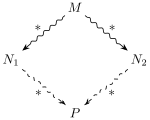
However far two runs of the same term have gone apart, they can be brought back together. So a term has at most one normal form: the order of the steps can change whether it is reached, not what it is. Church and Rosser proved this for the calculus in 1936.12 Not every term gets there. With for , the term has one redex, and the step gives back, for ever: nothing in the definition of -terms says what may be applied to what. The two combinators are terms too:
The step is two steps on , and the step is three. So every combinator term is a -term, and the two constants need no longer be taken as given.
Remark (looking back: combinators). Everything Chapter 1 did with combinators carries over. A definition is the term with the name left off, and unfolding it is one step for each parameter; with the and steps above, all three kinds of step there are . The Church–Rosser theorem there is the combinator version of the one here, and was proved after it. And is the Monster, the program that runs for ever: combinator terms didn’t say what may be applied to what either, and the Monster’s story reads unchanged in the new grain.
Theorem 3.5 (translation into combinators). Every -term translates to a term built from , , variables and application, with no in it, such that has the same free variables as and does the same thing to every argument: if is then for every . Conversely every combinator term is a -term, by the definitions of and above.
Proof. Translate innermost abstractions first. For a term containing no , define , “ abstracted over ”, by recursion on :
Then contains no and no , and
by induction on , one case for each clause:
If does not occur in : , and is .
If is : , and is .
If is : , and by the induction hypothesis on each half this runs to , which is .
Now take any -term, find an innermost abstraction (so has no ), and replace it by ; repeat until no is left. Each replacement preserves the free variables and the behaviour on arguments, so the result is . □
Remark (looking back: the Deduction Theorem as a compiler). You’ve seen the three clauses of before. The first writes a when the parameter is not used; the second writes the identity for the parameter itself; the third writes an to push the parameter through an application. Those are, case for case, the three cases of the proof of the Deduction Theorem in Chapter 2 — an axiom or hypothesis weakened by (I); the supposition itself, proved by the five-line proof of ; a modus ponens distributed by (II) — with the programs left on the lines. That chapter said the proof was the compiler that turns your \ta -> into combinators. Here it is, three lines long.
Theorem 3.6 (Turing completeness). Every function a Turing machine computes is computed by a closed -term, and every function a closed -term computes is computed by a Turing machine.
Proof. Chapter 1 proved this for combinator terms (Theorem 1.11), and the translation of the previous theorem converts each way without changing what is computed. □
That’s the order natural to these notes, which built the combinators first. History went the other way round. In 1936 Church proposed that “computable” should mean “definable by a -term”, and used that definition to show that no procedure decides whether two terms have the same normal form. That September Turing, who had never heard of the calculus, arrived at Princeton to study with Church, and in an appendix of 1937 he proved that his machines and Church’s terms compute the same functions (Turing, 1937a). Curry and his students showed the combinators equivalent to both.13 One theorem, proved by three groups of people about three notations: that’s a large part of why the history is confusing, and the end of the chapter draws it as a picture.
Example: factorial
Let’s send something ordinary the whole way round, so you can believe the three notations are one. Factorial, as you would write it on a whiteboard:
fact(n):
    if n = 0 then return 1
    else return n * fact(n - 1)
Four things in it are not in the combinator language: a parameter, a name that calls itself, a conditional, and arithmetic. Take them away one at a time. The parameter becomes a , which is what this section was for. Write , and for the test, the product and the predecessor, and use a boolean as its own conditional, so that “if then else ” is . Then
Nothing has really happened yet, because still occurs on the right-hand side, and a term may not refer to itself. So make the recursive call a parameter too:
mentions nothing but its own two parameters: give it the function to call and a number, and it does one layer of the work. What we want is a term with , a fixed point of . A constant added to the combinators, with the single step , is just what we want. So define . One step shows how it runs:
and on the right ’s parameter is again: the recursive call, ready to unfold once more when it is needed and no sooner.14 The arithmetic was combinators already: the numerals, addition and multiplication were all built from and , and the predecessor is Kleene’s. We keep the three as names only to keep the term on the page.
One thing remains, the two s, and the translation removes them. Write for the body, so that , and read as the application . The clause for an application splits it, the other two clauses finish each half, and with written for ,
twenty-six symbols, with still free. Abstract out of that by the same three clauses and every variable is gone:
where , and . There is not a variable, a parameter, a conditional or a recursive call anywhere in it, only , , three arithmetic constants and juxtaposition. Yet applied to runs to , by the and steps and the steps of the constants. A program you could have written in your first week sits on two constants in exactly this way, and so does every program you’ll ever compile.
Baker’s runbook, for what it’s worth, is code of the same kind. The rule she filed is a function of its supposition,
timeoutMeansTwice = \timeout -> chargedAgain (retried timeout)and the gateway’s “declined or approved” is a case with two branches; we’ll see the compiler check both in the next section.
3.5 The simply typed -calculus
On to the checker, and first to the Monster: the function that applies its argument to itself, applied to itself. In notation,
and each step gives back the term it started from. Self-application of this kind sank both of the logics these calculi were built for. The combinators came first: Schönfinkel had them in 1924 (Schönfinkel, 1924), and Curry, finding them again in the 1920s, built a logic on them in his thesis of 1929 (Curry, 1930). Church’s logic, with its variables bound by , followed in 1932. In 1935 Kleene and Rosser showed both inconsistent (Kleene and Rosser, 1935). The repair was the same in both cases: types. Curry gave his combinators types in 1934 (Curry, 1934), and Church gave his calculus types in 1940. Church’s typed calculus is the language of this section, the simply typed -calculus. Its types, contexts and judgements are those of the combinator checker: a type is a basic type or a function type ; a context lists the variables in scope with their types, ; and the judgement says that has type when its variables have the types gives them. Two of the rules are also the checker’s, for variables and for applications. The third is the Deduction Theorem, which the Hilbert system had to prove, adopted as a rule with the program written on:
Read (abs) as the checker reads a function definition: to check , add the parameter to the context with the type it is to have, check the body, and give the function the arrow type. If already declares an , rename the parameter first, since a context lists each variable once. Rule (abs) is the first typing rule we have met that changes the context: above the line there is one more variable in scope than below it, exactly as above an I bar there is one more open hypothesis than below it.
Remark (looking back: the missing rule). Chapter 1’s checker had no rule for a name with a parameter, and Chapter 2 showed that the rule it needed was a theorem. Rule (abs) is that rule, adopted. With it the compiler no longer has to compile anything to decide whether to say yes: it reads the definition as written. Adopting it types nothing new, since the translation turns any typed -term into a combinator term of the same type, with the types carried along. And the constants are gone. and are terms now, and (abs) gives them the very types Chapter 1 gave them,
Exercise 3.3 asks you to check this.
A typing of combinator terms was a list of lines under one context, which was enough because no rule changed the context. Rule (abs) does change it, so from now on a typing is a tree in which every node is a whole judgement, context included, and every bar is one of the three rules, premisses above and conclusion below. This is natural deduction in sequent style: the hypotheses available at each point are written at that point, rather than read off the leaves. Here is Baker’s rule, with and for the two runbook functions and for the supposition. With every context written out, the tree is too wide for the page, so here it is in two steps. First the application :
and then the rest, with that judgement, marked (1), as a premiss: The program at the root istimeoutMeansTwice, with , and for retried, chargedAgain and timeout. Now cover the programs with your thumb. Each node becomes a statement about formulas, with the hypotheses available there on the left of the . The tree is the one we drew for her rule, with those hypotheses written at every node: the leaves are what she was told and what she supposed, the two (app) bars are her two uses of modus ponens, and the (abs) bar is the (I) bar. Where the earlier tree put a bracket round the leaf , this one deletes from the context: two ways of recording the same discharge. In accepting the function, the compiler checked that tree.
Example: function composition
Here’s the typing of a program you’ve written in one form or another, \f -> \g -> \x -> f (g x), from the empty context. The body is checked in the context , written out at every node, and again in two steps to fit the page. First :
The top is routine: three look-ups and two uses of (app), each matching an argument’s type against the type a function expects. The (abs) bars shrink the context one declaration at a time, until at the root it is empty and the program is closed. Rub out the programs. The top is a proof of from the three hypotheses , and , by two uses of modus ponens. The three (abs) bars discharge , then , then . The first discharge alone gives from and : hypothetical syllogism, the rule that chains two implications. After all three, the formula at the root,
is hypothetical syllogism as a theorem, with nothing assumed. The compiler read your composition function as that proof.
Remark (looking back: hypothetical syllogism). Chapter 2 proved hypothetical syllogism twice, in seven lines each time: once from its two hypotheses, and once as the theorem above, where the first line was an instance of (II) with twenty letters and nineteen arrows that nobody would find by thinking about what implication means. Here the theorem is found and checked in three discharges.
The other connectives
The rules for , and get programs in the same way, and they are programs you know: a pair, a tagged union, the empty type. Baker’s morning was made of all three. At twenty past ten her evidence for was two pieces of evidence held together, an authorisation code and a capture id, and that pair is what a settled charge is in the payments database: one record with two fields, and to use either field you take it back out. At half past ten the gateway’s answer was a value with a tag on it, Declined with a reason or Approved with a code, and to use it she had to branch on the tag; the one thing checkout code must never do is treat an answer as approved without looking at the tag, and a tagged union is how a compiler makes that impossible. And when the logs disagreed she had, on paper, a value of the type that has none, which is why anything followed. Programs are full of all three. Pairs are tuples such as (min, max), and records and structs. Tagged unions are enums, Haskell’s Either, and Rust’s Result, a value or an error, which the compiler makes you handle both ways. The empty type is Haskell’s Void or Rust’s !, the type of a computation that never returns. A rule that introduces a connective builds a value of the type, so it is a constructor; a rule that eliminates one takes a value apart, so it is a pattern match. One thing changes on the page. A type theorist doesn’t write the pair type as , and I’ll follow the type theorists while we’re typing: the pair type is , the union , and the empty type , which the two traditions happen to share, along with .
Definition 3.7 (typing rules for , and ). is the pair type, (A, B); is the sum type, Either A B; is the type with no constructor, Void, of which there are no values; and is . The rules:
To build an you build both halves; to use one you take whichever half you need. To build an you build one side and say which; to use one you argue by cases. The case split, (E), is the one rule besides (abs) that puts a variable in scope: one in each branch, and only there. That is what “a different formula discharged in each branch” looked like on the tree. Nothing builds a , and if you ever have one you may conclude anything, which is what absurd :: Void -> a says. The whole language fits in one table: each connective, the type it is, how a value is built, how it’s taken apart.
| Connective | Type | Introduction (constructor) | Elimination (pattern match) |
|---|---|---|---|
, A -> B | application | ||
, (A, B) | , | ||
, Either A B | , | case with two branches | |
, Void | — | ||
, A -> Void | application |
That’s the central table of Part 1, and the one thing to carry away from it: the connectives of logic are the data types of a programming language, the introduction rules are their constructors, and the elimination rules are the pattern matches that take them apart. The first two columns are the same thing written by two trades, and the theorem below says what to do with the symbols when the programs are rubbed out: becomes and becomes , while and stay as they are.
Example 3.8 (three programs). Each of the following is a theorem, and here is the program that proves it.
: the program is , and its type is . In the context , (E2) gives and (E1) gives ; (I) gives the pair the type ; (abs) discharges . This is the tree we drew when learning to discharge, with and for its and , and the two bracketed leaves are the two occurrences of in the body. A variable used twice is a hypothesis discharged at two leaves; a variable used once, at one; and a parameter never used at all — , which is — is the receipt for a debt of nothing.
Contraposition, : the program is . In the context , two uses of (app) give , and three uses of (abs) give the type claimed. Baker’s modus tollens is this function applied to and the ledger’s .
Proof by cases: has type , which proves , and the two branch variables and are the two leaves and of the tree we drew for that formula, with and for its and , each in scope only in its own branch.
In each case the program is one you could have written without knowing what it proved: a function that swaps a pair; a function that composes a test with a function; a function that swaps the tags on a union. The types were there all along.
Theorem 3.9 (Curry–Howard).
(Erasure.) Take a typing of by (var), (app), (abs) and the rules for , and , delete every term, and write for and for throughout: (var) becomes a hypothesis, (app) an E bar, (abs) an I bar discharging the variable’s type, and each rule for , and the derivation clause for , or in the same position. The result is a derivation of , read as a formula, whose open hypotheses are among the types declared in , read the same way, a set we write .
(Decoration.) Take a derivation of , write for and for , choose a distinct variable for each open hypothesis and for each discharged one, and write terms upwards from the leaves: a variable at each leaf, an application at each E, a on the discharged variable at each I, and the matching constructor or pattern match at each other bar. The result is a typing of for some term , with declaring the open hypotheses.
In one line: for some term if and only if .
Proof. Put the typing rules beside the clauses that define derivations. Rule for clause, each derivation clause is the typing rule with the terms removed and the two symbols renamed: the premisses, the conclusions, and what each takes out of the context or out of are otherwise identical. In particular the free variables of an abstraction, , are computed as the (I) clause computes . Erasure and decoration are therefore the relabelling of combinator typings as Hilbert proofs in Theorem 2.4, with one more case per connective and one more for , and the proof is the same walk, down the typing for (i) and up the tree for (ii). □
A word about the renaming, since it is the only place the two readings of a rule differ on the page. A type theorist writes for the pair type and for the union, because a pair type has as many values as the product of its two halves and a union as many as the sum; a logician writes and , because those are the words. Church, Curry and Howard worked on the type side and Gentzen on the logic side, and nobody chose one notation for both, so the correspondence carries a small dictionary with it, for , for , and the same symbol for and . The symbols are the only thing that changes. From here on I write the type symbols in a typing and the logic symbols in a derivation, and when a formula is called a type, as in “a program of type ”, the rename has been done.
The new case, the , is the one that matters, and it is easy to undersell: “proofs resemble programs” says far less than the theorem does. The theorem says that a derivation in Gentzen’s system and a typing of a program with parameters, pairs, unions and case are the same tree with a column added; and that the rule which puts a parameter in scope and takes it out again is, column removed, the rule for supposing and discharging. Curry saw the Hilbert half of this in 1934; the half with and natural deduction is Howard’s, from 1969. That is why the observation carries both names.15
At work
None of this is a curiosity of logic books. Milner’s ML of 1978 is the typed -calculus with the types worked out by the compiler, offered with the promise that “well-typed programs cannot go wrong” (Milner, 1978); OCaml, F# and Haskell descend from it, and every lambda or closure in Java, C#, Swift, Rust or TypeScript is checked by rule (abs). The Glasgow Haskell compiler translates Haskell into a small typed -calculus of its own and can type-check that again after each optimisation, so that a compiler bug shows up as a type error. On the logic side, Church’s calculus of 1940 is the logic of the HOL family of proof assistants (HOL4, HOL Light, Isabelle/HOL), and in Coq (now Rocq), Lean and Agda a proof is a typed -term, in a richer calculus than this one, checked by a small kernel with rules like (var), (app) and (abs). Between them they have checked the seL4 operating-system kernel (Klein et al., 2009), the CompCert C compiler (Leroy, 2009), the Four Colour Theorem (Gonthier, 2008) and the Kepler conjecture (Hales et al., 2017). In each the trusted part is a type checker, and whoever wants the theorem does the hard part, finding the term.
So, finally, take the three rules (var), (app) and (abs), rub out the programs, and read what’s left. A supposition in force may be written down. From and , conclude . If follows on the supposition , conclude and drop the supposition. That’s how you were taught to prove an implication, in the first mathematics lecture you attended. Every time the checker reads a definition f x = ..., that is what it checks.
3.6 Normalisation and consistency
Hilbert hired Gentzen for something other than making proofs look like reasoning. The job was the programme that Part 3 tells in full: to prove, by arguments so elementary that nobody could doubt them, that mathematics could never derive a contradiction. The elementary arguments allowed were arguments about the shapes of written symbols — no appeal to infinite collections, no appeal to what the symbols were about — and natural deduction was built to make such arguments possible. Gentzen’s own account of the property he was after, from the same introduction as the quotation that opened the chapter:16
The Hauptsatz says that every purely logical proof can be reduced to a definite, though not unique, normal form. Perhaps we may express the essential properties of such a normal proof by saying: it is not roundabout. No concepts enter into the proof other than those contained in its final result, and they are necessarily used in arriving at that result.
A proof is roundabout when it takes what Gentzen called a detour: it establishes by I from proofs of and and at once takes back out by E1, or it establishes by I, discharging a supposition, and at once uses it on a proof of by E. In each case an introduction is met by its own elimination, and the proof would have been shorter without the pair. For the shortening looks like this, where is a proof of :
On the right, a copy of has been put in place of every leaf of , and the two bars have gone. Baker’s morning has a detour of exactly this kind. At ten past ten she proved the rule by supposing and discharging; at twenty to eleven, say, the gateway’s log gives her , a timeout at nine fifty-two, and she applies the rule to it. The reply she writes on the ticket does not mention the rule. It substitutes the evidence for straight into the reasoning that followed the supposition, and contains only facts about this charge — “no concepts other than those contained in its final result”. Look hard at that substitution, because you’ve seen it before.
Why they wanted normal proofs
Why should anyone care so much whether a proof is roundabout? Because of what a proof without detours cannot do. For and , a normal proof never invents material: every formula in it is a piece of its conclusion or of one of its open hypotheses. Now ask what a normal proof of from no hypotheses could look like. Every formula in it would be a piece of , and has no pieces; nor is there a rule that introduces it. There is nothing to build such a proof from. So if every proof can be rewritten into a normal one, nothing proves : normalisation gives consistency, by an argument about the shapes of proofs and nothing else. That is the kind of argument Hilbert wanted, and it is why Gentzen proved his normal-form theorem before he proved anything with it.
Hard to prove
The theorem was harder to come by than the argument for wanting it. Gentzen could prove that every derivation can be made normal for intuitionistic natural deduction, NJ, but not for its classical version. To cover classical logic he invented a third presentation of the rules, the sequent calculus, which Part 3 uses, and proved his Hauptsatz there. That proof covered the intuitionistic case as well, so he left the natural-deduction proof out of his thesis.17 The direct proof for natural deduction was published by Prawitz (1965), thirty years later. What the program view adds is not an easier proof of normalisation: the counting argument below works on terms exactly as it works on derivations. What it adds is a short road from normalisation to consistency, through the shape of a program that has stopped.
Definition 3.10 (reduction). A step rewrites, anywhere inside a term, an introduction met by its elimination:
There is no rule for , because has no introduction for it to meet. A term in which no step can be taken is in normal form, and, through the Curry–Howard correspondence, a derivation with no detour is a normal derivation.
These are the steps your interpreter takes: call a function, project a pair, branch on a tag. They also remove detours from proofs, and that is the last part of the correspondence, the part Howard credited to Tait. The two theorems about running combinators hold again, now for the whole language: a step never changes the type, which is called subject reduction because the term is the subject of the judgement ; and every typed program stops.
Theorem 3.11 (subject reduction). If and , then .
Proof sketch. The one new ingredient is a substitution lemma: if and , then . It is proved by going down the typing of and replacing every line that types by (var) with the typing of ; every later line is unchanged, since the rules look only at types. (On the proof side it is transitivity: a proof of spliced in for a hypothesis .) With that in hand, each step is one case. A step: came by (app) from and , and the first of these by (abs) from ; the lemma gives . A projection: came from , which came from . A case on : the conclusion came from , so , and from ; the lemma gives . A step inside a larger term replaces the lines for the subterm by lines of the same type. □
Theorem 3.12 (normalisation). Every typed term runs to a normal form. Equivalently: every derivation can be rewritten, by removing detours, into a normal derivation of the same formula from the same open hypotheses.
Proof for terms without . Give each type a degree, the height of its tree: a letter and have degree 1, and and have degree one more than the larger of the degrees of and . The degree of a redex is the degree of the type of the introduction form in it: the type of in , and the type of in or . By subject reduction a typed term stays typed as it runs, so these degrees stay defined.
Everything rests on one observation: a step on a redex of degree creates new redexes only of degree less than . A new redex appears only where an introduction form has come to stand under an elimination, and there are two ways for that to happen.
In a step , an occurrence of in that had an elimination applied to it (, or ) now has in its place. If is a or a pair, that is a new redex. Its introduction form has the type of , whose degree is less than that of .
The result of the step stands where the redex stood. If the result is a or a pair and the redex had an elimination applied to it, as in or , that is a new redex. Its introduction form has the type of the result in the case, and or in a projection: again of smaller degree.
Every other redex after the step was there before, perhaps copied: a step makes one copy of , with its redexes, for each occurrence of in .
Now take a typed term that is not in normal form. Let be the largest degree of a redex in it, and the number of redexes of that degree. Choose a redex of degree that contains no other redex of degree . One exists: if a redex of degree contains another, look at that one instead, and since the term is finite this stops. Take the step on . Then is gone; by the observation, no new redex of degree or more has appeared; and the copies made of the argument of contain no redex of degree , because contained none. So after the step either no redex of degree is left, and the largest degree has gone down, or the largest degree is still and there are redexes of it. Either way the pair has gone down, comparing first and second. That cannot happen for ever: can go down only finitely often, and while stays the same can go down only finitely often. So after finitely many steps no redex is left, and the term is in normal form. □
The argument is Prawitz’s, for derivations (1965), and Girard et al. (1989, chapter 4) give it for and much as here; Turing had found it for terms in the early 1940s, in a note that was published only in 1980.18 Notice that it is an argument about the shapes of terms and nothing else, the kind Hilbert asked for. It counts redexes and watches the count go down.
With the observation fails. A step on a puts a branch where the stood, and the branch can have any type at all: in
the new redex has the degree of the pair type of the branches, which need have nothing to do with the degree of , and the count can go up. A different method is needed, and Tait found one (1967): define, by induction on types, which terms are computable, show that every computable term normalises, and show that every typed term is computable. It covers every connective at once, and shows more: every order of steps reaches the normal form, not just a well-chosen one. Girard et al. (1989, chapters 6 and 10) give it. For terms with we take the theorem on trust.
Now watch it pay off, by the argument for wanting it. For and , a normal proof never invents material: every formula in it is a piece of its conclusion or of one of its open hypotheses.19 So if you want to know whether can be proved from nothing, you need only ask what a normal proof of from no open hypotheses could possibly look like. And a program that has stopped has a very particular shape.
Definition 3.13 (normal and neutral terms). A typed term is neutral if it is a variable, or an elimination applied to a neutral term: , , , , or , with neutral and the other parts in normal form. A term is in normal form (no step can be taken anywhere in it) exactly when it is an introduction form — , , or — whose parts are in normal form, or is neutral.
The “exactly when” is a small induction on the term, and the one thing it needs is types. Take a normal-form application . Its is in normal form and has an arrow type, and it is not a , or would be a redex. By induction is an introduction form or neutral; the only introduction form with an arrow type is a ; so is neutral, and then so is . The same argument handles a projection, whose argument cannot be a pair, and a case, whose argument cannot be a tag. The argument of an has type , which has no introduction form at all, so it too must be neutral. Exercise 3.11 asks for the cases in full. What matters is this: a neutral term is a chain of eliminations hanging off a variable, and that variable is free in it, since nothing in the chain binds it.
Lemma 3.14 (shape of closed normal forms). A closed typed term in normal form is an introduction form. Consequently there is no closed term in normal form whose type is a letter , and none whose type is .
Proof. A normal-form term is an introduction form or neutral, and a neutral term has a free variable, its head; so a closed one is an introduction form. An introduction form has type , or by the rule that introduces it, and none of those is a letter or . □
Theorem 3.15 (consistency). There is no closed term of type : . More generally, for every letter , .
Proof. By Curry–Howard it is enough to show that there is no closed term of type . Suppose . By normalisation, runs to a normal form . By subject reduction, ; and is closed, since no step of running creates a free variable. So is a closed normal-form term of type , and the shape lemma has just shown that there is no such term. The argument for a letter is the same with for . □
Read what we have shown. The logic of this chapter does not prove everything. It does not prove , and it does not prove any bare claim : whatever it proves has an arrow, an and or an or on the outside. So it proves things about how claims relate, and never a bare claim out of nothing. The argument used nothing about what the letters mean, no table, no notion of a formula being the case. It’s an argument about the shapes of strings, the kind Gentzen was hired to find. The route through programs is Howard’s, and it costs a page where Gentzen’s cost a thesis. Ask whether arithmetic proves everything, rather than the bare connectives, and you have the question Gentzen answered in 1936. It is the subject of Chapter 11, where the answer is of a different kind.
One more thing falls out of the shape lemma, and it’s worth having now.
Corollary 3.16 (disjunction property). If , then or .
Proof. By Curry–Howard there is a closed term of type . By normalisation and subject reduction it runs to a closed normal form of that type, which by the shape lemma is an introduction form: with , or with . □
In this logic you can’t establish “ or ” without establishing one of them and saying which, because a proof of a disjunction is a value with a tag on it. Baker’s log got away with “declined or approved” because the log was a hypothesis; a theorem would have had to say which. Hold on to this. Part 2 has a use for it.
Remark 3.17 (general recursion). Every language you use has recursion. Model it by a constant with the type for every and the step ; our factorial needed it. With it, has every type there is, and every letter included, so the consistency theorem fails; and it runs for ever, so normalisation fails with it. The two theorems go together, as they came together. Read as a logic, a language with general recursion proves everything, and a type in such a language promises only what the program does if it returns. The price of factorial is the consistency of the logic. Every language you use pays it, and pays it knowingly: the loop is worth more to a programmer than consistency is. A programmer who wants both must say in the type where the recursion is allowed to go, and that takes a logic with more to say than this one. The same price is why the checker’s yes, in the languages you use, means “safe” and never “correct”. The next chapter is about the gap between the two.
3.7 Fitch proofs
You’ve been drawing boxes all along, and it’s time to say whose they are. Jaśkowski’s system of 1934 wrote a proof not as a tree but down the page, one line after another as a Hilbert proof does, with one addition: a supposition opens a box, every line inside the box is reasoned under it, and the box closes at the line that discharges it, which stands outside. Fitch made the notation standard in 1952, drawing the box as a vertical bar with the supposition underlined at its top, and a proof drawn this way is called a Fitch proof.20 The boxes in which the combinator typings were written are Fitch proofs with the programs on, each a single box because nothing there was ever discharged.
Why are there two pictures, and why two names? The two inventions never met. Gentzen was in Göttingen and published in the Mathematische Zeitschrift. Jaśkowski was in Warsaw, among Łukasiewicz’s students, and published in English in the first volume of Studia Logica. The two men worked in different countries, wrote for different journals and moved in different circles, and neither ever heard from the other. The war then scattered the Warsaw school, and Jaśkowski’s paper reached the wider world only afterwards, through textbooks. Quine’s Methods of Logic set out its proofs in a form close to his in 1950, and Fitch’s book of 1952, whose preface credits both Gentzen and Jaśkowski, made the boxes standard. By then Gentzen had been dead for seven years. So nobody chose between the tree and the box. Two people answered the same question separately, and Theorem 3.19 at the end of this section says that their answers agree.21
A Fitch proof is a Hilbert proof that may open boxes inside its box, and it is a natural-deduction tree written down the page: a box is a subtree, and the nesting of boxes records what records.
Definition 3.18 (Fitch proof). A box has a head above a horizontal line and, below the line, a finite sequence of entries, each of which is either a formula, called a line, or another box, called a subbox. The head of the outermost box is a set of formulas. The head of a subbox is a single formula, its supposition, and its last entry is a line. The lines are numbered in one sequence down the page, whichever box they stand in, and a subbox is cited by the numbers – of its first and last lines:
| Line | Formula | Justification |
|---|---|---|
| 1 | reason | |
| i | reason | |
| j | reason | |
| n | reason |
A line or subbox is in scope at line if it comes before line and is an entry of a box that contains line : the box that line stands in, or one around it. So a subbox is in scope after it has closed, and the lines inside it are not.
Let be a set of formulas, the hypotheses. A Fitch proof of from is a box with head whose last entry is the line , and in which every line , in a subbox or not, is justified in one of the following ways, where “earlier” means “in scope at line ”:
(hyp) is a member of , or the supposition of a subbox that contains line ;
(E) there are earlier lines and such that is the formula ;
(I) is , and there is an earlier subbox with supposition whose last line is ;
(I) is , and and are earlier lines;
(E1, E2) some earlier line is , for some , or , for some ;
(I1, I2) is , and , or , is an earlier line;
(E) some earlier line is , and there are two earlier subboxes, one with supposition and one with supposition , each with last line ;
(E) is an earlier line.
No other kind of line is allowed. Theorem 3.19 below shows that has a Fitch proof from exactly when , so no new symbol is needed.
Put this beside Definition 2.2. The outer box is the same box, with the hypotheses above the line and the lines below it. (hyp) is the hypothesis clause, with the supposition of every box around a line counted among that line’s hypotheses, and (E) is modus ponens, word for word. The axiom clause has gone: the rules that open subboxes do its work. Everything new comes with the subbox, and so does the one restriction. A line inside a subbox was reasoned under its supposition, so once the subbox has closed, nothing outside it may cite that line. Only the subbox as a whole may be cited, and only by (I) and (E), the two rules that discharge.
Each line has a context: together with the suppositions of the subboxes that contain it. A line with context stands for the judgement . Read that way, each clause is one of the typing rules of §3.5 with the terms deleted: (hyp) is (var), (E) is (app), and (I) is (abs), whose premiss is the last line of a subbox with supposition .
Baker’s rule once more, drawn earlier as a tree and now as a box:
| Line | Formula | Justification |
|---|---|---|
| 1 | (hyp) | |
| 2 | (hyp) | |
| 3 | (E) 2, 1 | |
| 4 | (hyp) | |
| 5 | (E) 4, 3 | |
| 6 | (I) 1–5 |
It is her six lines of the opening page with the justifications formalised, and it is the typing tree of §3.5 with the programs rubbed out and the tree written down the page. Lines 2 and 4 stand inside the subbox and cite hypotheses from the head of the outer box, which is around them. Line 6 stands outside, and cites the subbox as a whole.
Here, then, is the theorem the history asks for. Gentzen’s trees and Jaśkowski’s boxes are two notations for one system: they prove the same things from the same hypotheses, and they prove them by the same steps.
Theorem 3.19 (trees and boxes). For every set of formulas and every formula , the following are equivalent:
: some tree derivation has conclusion and all its open hypotheses in ;
has a Fitch proof from .
Moreover, the translations both ways go step by step: each bar of a tree becomes a line justified by the same rule, and each line of a Fitch proof not justified by (hyp) becomes a bar of the same rule.
Proof. Left to right. We show, by induction on a tree derivation with conclusion , that has a Fitch proof from every that contains . One fact is used throughout: the entries of a Fitch proof from may be copied, renumbered, into any box at a place where every member of is a hypothesis or the supposition of a box around them. Each (hyp) line is still justified, and every other line cites only lines and subboxes of the copy, which are still in scope.
A one-node tree : here , and the proof is the single line , by (hyp).
(E), (I), (E), (I) and (E): the open hypotheses of each immediate subtree lie inside , so inside , and by induction each premiss has a Fitch proof from . Copy their entries one after another into a box with head , and add the conclusion as a line, justified by the rule from the last lines of the copies.
(I), with immediate subtree concluding : , so by induction has a Fitch proof from . Copy its entries into a subbox with supposition , inside a box with head , and add after the subbox, by (I).
(E): the same, with a Fitch proof of from first and then one subbox for each branch, followed by the conclusion, by (E).
Right to left. Write for the context of line . Going down the page, we build for each line a tree with conclusion and open hypotheses inside . A line justified by (hyp) gets the one-node tree , and . Any other line cites earlier lines and subboxes. A line in scope at line stands in no box that does not also contain line , so . The last line of a subbox in scope at line , with supposition , has . Put the trees already built for the cited lines above a bar for the matching rule. For (I) the bar removes from the open hypotheses, and for (E) it removes from one branch and from the other, so the open hypotheses of the new tree lie inside . The last line of the proof has context , and its tree witnesses . Both constructions add one line for each bar, or one bar for each line, under the same rule, which is the last part of the theorem. □
Programs can be written in the boxes too, and then (abs) is a box inside a box. To type , open an inner box whose declaration is , type the body inside it, and close the box. The line after it, , is written outside the box, because outside the box is not in scope. A line may use a declaration from its own box or from any box around it, and nothing written inside a box that has been closed. That’s the scope rule of a programming language, and it is why proof assistants display proofs in this way. For typing, though, these notes use the trees of §3.5. In a box the context of a line is not written on the line: it has to be read off the boxes around it, and a term such as inside a box has a free variable whose declaration is somewhere above. In sequent style every judgement carries its whole context, and each step can be checked without looking anywhere else.
Trees, sequent-style trees and boxes are three notations for one object, and the theorem is the licence to move between them without comment. We draw trees when the shape of an argument is the point, and boxes when a proof is long and best read from top to bottom.
3.8 History
Three chapters have told a history in footnotes, which is the right way to read it and the wrong way to remember it. It has nearly twenty people in it, Curry and Church twice each, doing the same things under different names. As one picture it’s a diamond, and it converges.
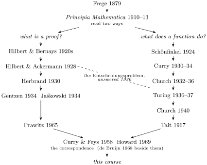
At the top is one book, read two ways. Hilbert read Principia and saw that a proof could be written down as a list and checked; so proof theory, the Deduction Theorem, and Gentzen’s rebuilding of the list as a tree. Schönfinkel, Curry and Church read it and saw mechanical instructions for rewriting formulas, above all for handling variables, and asked what a function does when it is applied; so the combinators, the , and, once Turing had asked the question in his own way, the theory of computation. The two edges first touch in 1936. Hilbert and Ackermann had asked, on the left, for a procedure that decides, of any formula, whether it is provable; Church and Turing, on the right, showed that there is none. They meet at the bottom, when Curry noticed that the types of his combinators were Hilbert’s axioms, and Howard, eleven years later, that the typing rules for , pairs and unions were Gentzen’s, and that running was normalising. Below that is this course, which has walked the diamond backwards.
Four pairs of names are confused more often than not, and one sentence each will settle them. Curry and Church built two calculi for the same doomed logic, one with constants and one with ; one paradox broke both, and each repaired his own with types, Curry in 1934 and Church in 1940. Church and Turing gave two definitions of “computable” that are one theorem, and the thesis named after both is the claim that the theorem is about everything.22 Gentzen and Jaśkowski invented “suppose” in the same year without knowing of each other, one as a tree and one as a box. Curry and Howard saw the two halves of one correspondence thirty-five years apart, Curry for the Hilbert system and the combinators, Howard for natural deduction and the -calculus — and Howard saw also that running was normalising, which Prawitz and Tait had just proved on the two sides, two years apart, with one proof.
| Who | When | What |
|---|---|---|
| Frege | 1879 | proofs as gap-free chains; axioms (I), (II) |
| Whitehead & Russell | 1910–13 | the whole of mathematics, by rule |
| Hilbert & Bernays | 1922– | proofs as objects; proof theory |
| Schönfinkel | 1924 | and suffice |
| Hilbert & Ackermann | 1928 | the textbook; the Entscheidungsproblem |
| Herbrand | 1930 | the Deduction Theorem |
| Curry | 1930–34 | combinatory logic; the types of , |
| Church | 1932–36 | the -calculus; an unsolvable problem |
| Gentzen, Jaśkowski | 1934 | natural deduction; the Hauptsatz |
| Turing | 1936–37 | the machine; equivalence with |
| Church | 1940 | the simply typed -calculus |
| Curry & Feys | 1958 | types of combinators are axioms, in print |
| Prawitz; Tait | 1965; 1967 | normalisation, both sides |
| Howard | 1969 | the correspondence for and NJ |
Summary
Natural deduction is the Hilbert system with every axiom read backwards through the Deduction Theorem: nine rules for going on and no way to start except by supposing, and the whole cost of the theorem is the cost of discharging a supposition. Its derivations are trees, and a bracket round a leaf is a receipt for a supposition paid off. NJ proves exactly what the Hilbert system proves (Theorem 3.3). Decorated with programs, a derivation is a typing in the simply typed -calculus (Theorem 3.9): a hypothesis is a variable, I is , E is application, and the other connectives are your data types, their introduction rules the constructors and their elimination rules the pattern matches. The untyped calculus compiles to and by the theorem’s own construction and computes whatever a Turing machine computes. Running a program is removing detours from a proof. What the checker said survives the run (subject reduction), and every typed program stops (proved here by counting redexes, except for ). A stopped closed program is a constructor, so the logic proves no letter and no — the theorem Gentzen was hired to prove, by the route Howard noticed thirty-five years later — and a proof of or always says which.
Safe is not correct. Nothing we care about — a sorted list, a transitive order, a discount on every day of the sale — is proved from no hypotheses. By the consistency theorem, nothing with a bare claim at the top ever is. Such things are proved from a specification, a set of sentences about lists, orders or sales taken as hypotheses. And a specification says for all — every payment, not the one on Baker’s ticket; every day of the sale — which no formula of this chapter can say.
Exercises
Exercise 3.1. Draw derivations, in Gentzen’s notation, of the schemas (fst) , (either) and (absurd) with no open hypotheses, and compute for each from the clauses. Then decorate the derivation of (either) with a program, and say which Haskell function it is.
Exercise 3.2. Baker’s log says the gateway declined the attempt or approved it; the runbook says a declined attempt is written to the ledger, and an approved attempt is written to the ledger only once its capture is posted, which it has been. Write the letters, draw the derivation of , and compute its open hypotheses. Then give the program.
Exercise 3.3. Give typings of and of by (var), (app) and (abs), and confirm that the types are and , the ones Chapter 1 gave and . Then run and count the steps.
Exercise 3.4. Run for three steps. Then run , first blindly and then renaming the bound first, and say which answer is the one meant.
Exercise 3.5. Translate , the numeral , into combinators by the three clauses of , innermost first, and check that the result applied to and runs to .
Exercise 3.6. Give derivations of and of , as trees, and then write the program each one is.
Exercise 3.7. Find a closed program of type , and give the derivation it is, a proof of .
Exercise 3.8. Find a closed program of type , and say which formula it proves.
Exercise 3.9. Try to find a closed program of type , for a letter . Say where every attempt sticks. Keep your attempt; Part 2 returns to this formula.
Exercise 3.10. The proof that natural deduction and the Hilbert system agree turns Chapter 2’s Hilbert proof of hypothetical syllogism, , into a derivation; decorated, it is the program with and written as -terms. That derivation has detours. Run the program to normal form and compare it with the typing of the composition function in §3.5.
Exercise 3.11. Prove in full the “exactly when” in the definition of normal and neutral terms: show by induction on a typed term in normal form that it is an introduction form with normal-form parts or neutral, giving the cases for and carefully, and say where the type is used.
Reading
Gentzen (1934) is the original, and its introduction, in Szabo’s translation, is four pages anyone can read. Girard et al. (1989, chapters 2–4) is the text behind the second half of this chapter: natural deduction, the identification of proofs with programs, conversions as the removal of detours, and the normalisation theorem proved in full for and . It is short, free online, and the right next thing to read. Prawitz (1965) is the book that made normal proofs a subject; Howard (1980) is the correspondence as Howard wrote it down in 1969; Wadler (2015) is the story told to programmers, with the diamond drawn differently. Menzler-Trott (2007) is Gentzen’s life, and von Plato (2008) is the manuscript in Zürich. Next, Chapter 4: for all, and proving from a specification.
References
- Henk Barendregt. The impact of the lambda calculus in logic and computer science. Bulletin of Symbolic Logic, 3(2):181–215, 1997.
- Alonzo Church. A set of postulates for the foundation of logic. Annals of Mathematics, 33(2):346–366, 1932.
- Alonzo Church. An unsolvable problem of elementary number theory. American Journal of Mathematics, 58(2):345–363, 1936.
- Alonzo Church. Review of A. M. Turing, On computable numbers, with an application to the Entscheidungsproblem. Journal of Symbolic Logic, 2(1):42–43, 1937.
- Alonzo Church. A formulation of the simple theory of types. Journal of Symbolic Logic, 5(2):56–68, 1940.
- Alonzo Church and J. Barkley Rosser. Some properties of conversion. Transactions of the American Mathematical Society, 39(3):472–482, 1936.
- Haskell B. Curry. Grundlagen der kombinatorischen Logik. American Journal of Mathematics, 52:509–536, 789–834, 1930.
- Haskell B. Curry. Functionality in combinatory logic. Proceedings of the National Academy of Sciences of the USA, 20(11):584–590, 1934.
- Frederic B. Fitch. Symbolic Logic: An Introduction. Ronald Press, New York, 1952.
- Robin O. Gandy. An early proof of normalization by A. M. Turing. In J. P. Seldin and J. R. Hindley, editors, To H. B. Curry: Essays on Combinatory Logic, Lambda Calculus and Formalism, pages 453–455. Academic Press, London, 1980.
- Gerhard Gentzen. Untersuchungen über das logische Schließen I, II. Mathematische Zeitschrift, 39:176–210, 405–431, 1934. Appeared 1934–35; English translation in The Collected Papers of Gerhard Gentzen, ed. M. E. Szabo, North-Holland, 1969.
- Jean-Yves Girard, Yves Lafont, and Paul Taylor. Proofs and Types, volume 7 of Cambridge Tracts in Theoretical Computer Science. Cambridge University Press, 1989. Free online.
- Georges Gonthier. Formal proof—the four-color theorem. Notices of the American Mathematical Society, 55(11):1382–1393, 2008.
- Thomas Hales et al. A formal proof of the Kepler conjecture. Forum of Mathematics, Pi, 5:e2, 2017.
- William A. Howard. The formulae-as-types notion of construction. In J. P. Seldin and J. R. Hindley, editors, To H. B. Curry: Essays on Combinatory Logic, Lambda Calculus and Formalism, pages 479–490. Academic Press, London, 1980. Written in 1969.
- Paul Hudak, John Hughes, Simon Peyton Jones, and Philip Wadler. A history of Haskell: being lazy with class. In Proceedings of the Third ACM SIGPLAN Conference on History of Programming Languages (HOPL III), pages 12–1–12–55, 2007.
- Stanisław Jaśkowski. On the rules of suppositions in formal logic. Studia Logica, 1:5–32, 1934.
- Stephen C. Kleene and J. Barkley Rosser. The inconsistency of certain formal logics. Annals of Mathematics, 36(3):630–636, 1935.
- Gerwin Klein et al. seL4: Formal verification of an OS kernel. In Proceedings of the 22nd ACM Symposium on Operating Systems Principles (SOSP), pages 207–220, 2009.
- Xavier Leroy. Formal verification of a realistic compiler. Communications of the ACM, 52(7):107–115, 2009.
- Paul Lorenzen. Einführung in die operative Logik und Mathematik. Springer, Berlin, 1955.
- John McCarthy. History of LISP. ACM SIGPLAN Notices, 13(8):217–223, 1978.
- Eckart Menzler-Trott. Logic’s Lost Genius: The Life of Gerhard Gentzen, volume 33 of History of Mathematics. American Mathematical Society and London Mathematical Society, 2007. Translated by Craig Smoryński and Edward Griffor.
- Robin Milner. A theory of type polymorphism in programming. Journal of Computer and System Sciences, 17(3):348–375, 1978.
- Francis Jeffry Pelletier. A history of natural deduction and elementary logic textbooks. In John Woods and Bryson Brown, editors, Logical Consequence: Rival Approaches, volume 1, pages 105–138. Hermes Science, Oxford, 2000.
- Dag Prawitz. Natural Deduction: A Proof-Theoretical Study. Almqvist & Wiksell, Stockholm, 1965.
- J. Barkley Rosser. Highlights of the history of the lambda-calculus. Annals of the History of Computing, 6(4):337–349, 1984.
- Moses Schönfinkel. Über die Bausteine der mathematischen Logik. Mathematische Annalen, 92:305–316, 1924.
- William W. Tait. Intensional interpretations of functionals of finite type I. Journal of Symbolic Logic, 32(2):198–212, 1967.
- Alan M. Turing. Computability and -definability. Journal of Symbolic Logic, 2(4):153–163, 1937a.
- Alan M. Turing. The -function in --conversion. Journal of Symbolic Logic, 2(4):164, 1937b.
- Jan von Plato. Gentzen’s proof of normalization for natural deduction. Bulletin of Symbolic Logic, 14(2):240–257, 2008.
- Philip Wadler. Propositions as types. Communications of the ACM, 58(12):75–84, 2015.
Notes
Gentzen’s thesis, Untersuchungen über das logische Schließen (Gentzen, 1934), was written in 1932–33 under Paul Bernays, who had been Hilbert’s collaborator on proof theory since 1917 and was writing the Grundlagen der Mathematik with him. In April 1933 Bernays was dismissed from the university under the new civil-service law, because he was a Jew; he left for Zürich the next year, and the thesis was examined by Hermann Weyl, who was himself about to leave. Gentzen went on writing to Bernays in Zürich for the rest of his life — drafts, the consistency proof for arithmetic of 1936, the ordinal that measures it — in letters that discuss nothing but mathematics, through the years in which he joined the SA and then the Party and in which Bernays could not have come back. The letters are in Menzler-Trott (2007), and I leave the reader to draw the conclusion. From 1935 Gentzen was Hilbert’s assistant. He taught in Prague from 1943, was arrested there with the rest of the German faculty in May 1945, and died in the prison on 4 August 1945, of starvation; he is said to have gone on working, in his cell, on the consistency of analysis. ↩
Gentzen (1934, p. 68), in Szabo’s translation. Natural deduction was invented twice in 1934. Stanisław Jaśkowski in Warsaw, provoked by the complaint of Łukasiewicz’s seminar quoted in Chapter 2, printed a system of the same kind the same year (Jaśkowski, 1934), having presented it to the First Polish Mathematical Congress in 1927; neither knew of the other. Gentzen wrote his proofs as trees and Jaśkowski wrote his in boxes, and the boxes, as the end of this chapter explains, are the ones you have been drawing all along. ↩
“The introductions represent, as it were, the ‘definitions’ of the symbols concerned, and the eliminations are no more, in the final analysis, than the consequences of these definitions” (Gentzen, 1934, p. 80). Lorenzen named this the inversion principle in 1955, and Prawitz made it exact; it is the seed of the proof theory at the end of this chapter. ↩
Some books let a rule discharge a chosen subset of the open copies rather than all of them, or forbid discharging a formula that does not occur. Nothing derivable changes under either convention; the one here is the simplest to state and matches what a function’s parameter does, as we’ll see. ↩
The trees are Gentzen’s, root at the bottom, as he drew them and as no computer scientist draws any other tree. The square brackets round a discharged leaf are Prawitz’s, from the book (1965) that made natural deduction a subject again thirty years after Gentzen; Gentzen himself marked a discharged formula only with its number. I use for the moment to keep the new relation apart from the Hilbert system’s , until we have shown that the two agree. ↩
The language Haskell is named after Haskell Curry, with his widow’s permission. After a talk about it at Penn State, Virginia Curry told one of its designers: “You know, Haskell actually never liked the name Haskell” (Hudak et al., 2007). ↩
Church was born in Washington in 1903 and spent almost his whole working life at two universities: Princeton, as student and then professor, until 1967, and then UCLA, where he taught until 1990, when he was eighty-seven. A childhood accident with an air gun had left him blind in one eye; his blackboard was nonetheless remembered as immaculate. He was exceedingly polite and exceedingly careful. He protected papers he valued with a coat of Duco cement, a clear household glue, and he read science-fiction magazines and wrote to their editors when they got something wrong. He was a founder of the Journal of Symbolic Logic in 1936 and edited its reviews until 1979, and he supervised thirty-one doctorates. Among them were Kleene, Rosser and Turing; Martin Davis; Michael Rabin and Dana Scott, who shared a Turing Award, a prize named after an earlier student of their supervisor; and Raymond Smullyan, of the mockingbirds, who had once performed in Chicago nightclubs as a stage magician called Five-Ace Merrill. ↩
Python’s
lambdacame from Church by way of Lisp. John McCarthy, designing Lisp in 1958, needed a notation for functions passed as arguments, and “it seemed natural to use the -notation of Church”, from Church’s little book of 1941. Twenty years later he added: “I didn’t understand the rest of his book, so I wasn’t tempted to try to implement his more general mechanism for defining functions” (McCarthy, 1978). In 2005 Python’s designer proposed takinglambdaout of the language, because “most Python users are unfamiliar with Lisp or Scheme, so the name is confusing”. It stayed. ↩Church used it in 1936 to exhibit a problem no procedure can settle (Church, 1936), and gave it types in 1940. Why ? Whitehead and Russell had written the function with body as , with a hat; the story told by Church’s student Rosser is that a typesetter could not set the hat over the letter and moved it in front, where it became a capital lambda and then a small one (Rosser, 1984). Church himself, asked late in life, said the choice had been arbitrary. Barendregt tells both versions and believes neither entirely (Barendregt, 1997). The three forms are in Church (1940, §1), where he also proves that and are -terms. ↩
Getting this wrong is a rite of passage, and the first Lisp got it wrong. A function passed as an argument looked up its free variables where it was called rather than where it was written, so a variable of the caller could capture one of the function’s own. McCarthy later wrote: “I must confess that I regarded this difficulty as just a bug and expressed confidence that Steve Russell would soon fix it” (McCarthy, 1978). Lisps went on looking variables up that way for many years; Scheme, in 1975, was the first to do what clause 5 says by default. ↩
Turing’s doctoral thesis was written under Church (1938), and Church’s two earlier students, Kleene and Rosser, had done most of the work of showing that the calculus could compute anything at all. Gödel, in Princeton at the time, was not persuaded that -definability captured “computable” until he read Turing’s paper, and then was. The name “Turing machine” is Church’s, from his review of Turing’s paper (Church, 1937); Turing had called them computing machines. ↩
In the untyped calculus need not be added: Curry’s satisfies by two steps, and Turing gave one of his own in 1937, , which does the same in a form that reduces to rather than merely to something equal to it (Turing, 1937b). Both are the Monster’s self-application put to work, which is why neither has a type (§3.6). ↩
Howard’s notes (1980) credit a talk of Tait’s in 1967 for the part of the correspondence that the next section is about: that running a program is Gentzen’s normalisation. “Simply typed” is Church’s phrase from 1940, and the “simple” is the simple theory of types, Ramsey’s 1926 simplification of the ramified theory of Principia, in which a function’s type had recorded not only what it took and returned but at what stage it had been defined. It has nothing to do with difficulty. ↩
Gentzen (1934, p. 69). His word is Umweg, a detour; Hauptsatz means the main theorem. ↩
In 2005 Jan von Plato found, among Bernays’s papers in Zürich, a handwritten version of the thesis that contains a detailed proof of normalisation for natural deduction, in the form that later became standard (von Plato, 2008). Gentzen had the proof and set it aside: the sequent calculus handled classical and intuitionistic logic at once, so there was no need to print it. ↩
Gandy (1980), where Gandy prints Turing’s note with a commentary. ↩
With and the reductions above are not quite enough for this. In
no step can be taken, because meets a rather than a pair, yet the pair type in the middle need not be a piece of anything at either end. Prawitz adds permutative conversions, which move the inside the branches, and similar ones for ; with them the property holds for all the connectives (Prawitz, 1965). The consistency proof below does not need it: it goes through the shape of closed terms. ↩
Frederic Fitch, at Yale; Symbolic Logic: An Introduction, 1952. Fitch’s bars are Jaśkowski’s boxes with their right-hand sides rubbed out. Every proof assistant in use presents its proofs this way, with “suppose” as
introorassumeand the box as indentation, and so does the scope rule of every compiler: a parameter is in scope inside the function and not outside it. ↩The two were “never in contact with one another”, in the words of the standard history, Pelletier (2000), which also traces the textbooks. Jaśkowski had shown his system to the Polish Mathematical Congress in 1927, but the published proceedings record the talk by title only. ↩
Neither of them named it. Kleene called it “Church’s thesis” in 1952, and added Turing’s name in 1967. ↩