Chapter 5: Second-Order Logic

Okafor reviews code for a bank. A pull request from another team changes a helper that runs whenever the bank’s two offices hold different copies of the same customer’s record and one of them has to win. The helper is four hundred lines long, and its type is

pick :: a -> a -> a

The question on the review ticket is the one a bank cares about: can this change corrupt a record, by mixing the fields of two records, say, or blanking a card number? Okafor approves it after reading one line, the type.

Here is her reasoning. The type says that pick works for every type a: whatever a record is, it takes two of them and returns one. It was written without knowing what an a is, so it can’t look inside one, can’t change a field, and can’t build a new record, because nothing it was given says how. The only as it has are the two it was handed, so what it returns is one of those, as it arrived. Whatever the four hundred lines do, they can’t corrupt a record.¹ The one thing left to review is which of the two it keeps, and a single test settles that.

That’s a theorem about a program, read off its type, and the type is a quantifier over types: pick has the type $\mathrm{\Pi }a(a\to a\to a)$. The chapter begins with the logic that quantifier belongs to.

Chapter 4’s quantifiers range over things. Let one range over propositions instead and you get second-order logic, in which a schema becomes a single theorem and the connectives $\wedge$, $\vee$ and $\mathrm{\perp }$ can be defined from $\to$ and $\mathrm{\forall }$. The quantifier is of a kind Russell banned, so when the logic is on the page its consistency is an open question.

Then the programs go back on, as they did in Chapter 4, and what comes out is something you already use: generics, the a in length :: [a] -> Int, with the side conditions as two compiler error messages, and in full the polymorphic $\lambda$-calculus, also called System F. Girard’s proof that its programs stop answers the logic’s question, and gives Okafor’s argument as a theorem. Pushed one step further, to a type of all types, the system collapses, as Church’s logic did in Chapter 1 before types repaired it.

5.1 Quantifying over propositions

The first-order quantifiers range over things: kinds, drivers, days. Look back at the propositional theorems, though, and you’ll find a quantifier of another kind that nobody wrote down. The theorem $p\to p$ was never about $p$ in particular. Its proof works with any formula at all in the place of $p$, and that is why the Hilbert system states its axioms as schemas, with Greek letters standing for every formula.

A schema is a claim about all formulas made one instance at a time, which is Ivanova’s forty letters from Chapter 4 again. The cure is the same as before. Let a quantifier range over propositions, and write the claim once: $\mathrm{\forall }X(X\to X)$, “whatever proposition $X$ is, $X$ implies $X$”.

The variable $X$ needs a symbol of its own. The propositional letters $p,q,r$ are constants: each stands for one fixed claim, and nothing can bind it. A variable for propositions is as different from a letter as the variable $x$ is from the constant $\mathsf{cam}$, so we write propositional variables differently, as $X,Y,Z$.

The two quantifier rules are the first-order ones with propositions in the place of things: ($\mathrm{\forall }$I) generalises over a proposition nothing open says anything about, and ($\mathrm{\forall }$E) uses the result at a particular one.

5.2 The connectives, defined

The logic has $\to$ and $\mathrm{\forall }$ and nothing else, and needs nothing else, because $\wedge$, $\vee$ and $\mathrm{\perp }$ can be written with those two. Say what you can do with a conjunction: from $A\wedge B$ you can conclude every claim that follows from $A$ and $B$ together. Then let that be the definition.

Each connective is defined by its elimination rule:

• $A\wedge B$ says “whatever follows from $A$ and $B$ together, follows”;

• $A\vee B$ says “whatever follows from $A$ and also from $B$, follows”, which is proof by cases;

• $\mathrm{\perp }$ says “everything follows”.

So propositional NJ sits inside this one, built from $\to$ and $\mathrm{\forall }$ alone.

Higher-order logic

Second-order propositional logic quantifies over propositions. Higher-order logic goes the whole way: over properties of things, relations between them, properties of properties, and functions of every type. Its language is the simply typed $\lambda$-calculus itself, with a type $o$ of propositions and a type $\iota$ of things, so that a property of things is a term of type $\iota \to o$, and a variable $P$ of that type can be bound by $\mathrm{\forall }P$. This is Church’s simple theory of types (Church, 1940), the logic for which he typed his calculus. In it, induction on the natural numbers is one sentence,

where first-order logic needs a schema, one axiom for each formula.

The power has a price: Chapter 16 shows that once the quantifiers are read as ranging over all properties, no proof system whose proofs can be checked mechanically captures that reading, even for second-order logic.

Impredicativity

Look at ($\mathrm{\forall }$E) once more. The formula $B$ put in for $X$ may be any formula at all, including $\mathrm{\forall }XA$ itself: $\mathrm{\forall }X(X\to X)$ may be used at $\mathrm{\forall }X(X\to X)$, and $\mathrm{\perp }$, which is $\mathrm{\forall }XX$, at $\mathrm{\perp }$. A quantifier over all propositions ranges over a collection that includes the proposition it is helping to form. Definitions of that kind are called impredicative, and Russell banned them from Principia for fear of the self-application that produced the paradoxes.

So we have to ask whether this logic is consistent. For first-order logic the answer came from programs:

1. decorate the derivations;

2. run them;

3. look at what they stop at.

Do the same here.

5.3 Generics

Decorate a second-order derivation as Chapter 4 decorated a first-order one:

• the bars for $\to$ become $\lambda$ and application, as before;

• a ($\mathrm{\forall }$I) bar over $X$ becomes a type abstraction $\mathrm{\Lambda }a.M$, a program that takes a type and returns a program;

• a ($\mathrm{\forall }$E) bar at $B$ becomes an instantiation $M[B]$, which hands it one.

The formulas become types, with the usual renaming: a propositional variable $X$ becomes a type variable $a$, a type nobody has chosen yet, and $\mathrm{\forall }X$ becomes $\mathrm{\Pi }a$, the $\mathrm{\Pi }$ of dependent types with types in the place of things. The two theorems of Example 5.2 decorate to

What has come out is something you’ve been writing for years, and Okafor’s type. $\mathrm{\Pi }aA$ is the type of a program that works for every type $a$, and the rules are ($\mathrm{\Pi }$I) and ($\mathrm{\Pi }$E) of Chapter 4’s dependent types with types in the place of things,

where $B$ may mention only type variables declared in $\mathrm{\Gamma }$. The context is the same stack, and running is one more step, $(\mathrm{\Lambda }a.M)[B]⇝M[B/a]$.

The type of length is [a] -> Int, and the a in it is a parameter, a type nobody has chosen yet. Haskell leaves the quantifier out, and writes it forall only when asked. Written in, it reads $\mathit{length}:\mathrm{\Pi }a([a]\to \mathit{Int})$, so length is a function that works for every element type at once.

Without a way to say for every you’d have three options.

1. The first is one copy per element type,

   lengthOfIntList,   lengthOfStringList,   lengthOfBoolList,   …

   which is Ivanova’s forty letters from Chapter 4 once more.

2. The second is to give it the type [Object] -> Int and cast on the way in and out. Java made people do that until 2004, and a wrong cast is caught only when the program runs.

3. The third is to turn the checker off for that part of the program.

With the quantifier you write the code once and check it once, for every type, and that’s why map, filter, sort and every container you’ve used have one in their types. The logic got there first: a generic function is a proof of a schema, written once.

The side condition on ($\mathrm{\forall }$I), the one Chapter 4 ran to $\mathrm{\perp }$, turns up as an error message. Try

f :: a -> b
f x = x

and GHC answers couldn’t match expected type b with actual type a, adding that a is a rigid type variable bound by the signature.

Here’s what happened in the stack. The signature declared $a$ and $b$ and promised a program that works for both separately. The body can only be typed if $a$ and $b$ are the same, which means a hypothesis about $a$ is still in force when the checker reaches the ($\mathrm{\Pi }$I) that would pop it. Rigid is the compiler’s word for declared and not last, a variable the context has fixed and you may not generalise over.

{-# LANGUAGE ExistentialQuantification #-}
data Counter = forall a. MkCounter a (a -> a) (a -> Int)

intCounter  = MkCounter (0 :: Int)   (+1)    id
listCounter = MkCounter ([] :: [()]) (():)   length

tick3 :: Counter -> Int
tick3 (MkCounter s step out) = out (step (step (step s)))

The generic quantifier, side conditions and all, has been at work every time the compiler has read a definition with a type variable in it. It is second-order logic with its programs on, and the next section writes the calculus down in full.

5.4 The polymorphic $\lambda$-calculus

Here is the calculus the section on generics used informally.

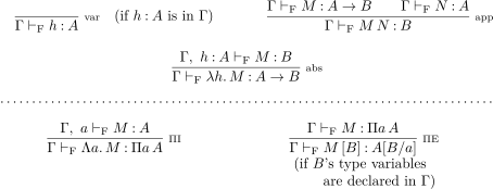
The rules for $\mathrm{\Pi }$ are those of dependent types with the domain changed from things to types, and the context is the same stack. There are no pairs, no unions and no $\mathrm{\perp }$, for the reason the logic has already given: they can be defined.

Erasure and decoration go through as before, so a formula without letters is derivable from no hypotheses exactly when a closed program of the corresponding type exists. (The letters are the logic’s constants, and the calculus has no counterpart for them, just as it has no types like Int built in.)

Data types, defined

Decorate the derivations in the proof of the proposition on the connectives, and the definitions of $\wedge$, $\vee$ and $\mathrm{\perp }$ become programs, with $a$ for $X$ and $C$ for the result type:

In the line for ($\vee$E) the braces hold the usual two branches, $\mathit{Left}h\Rightarrow Q$ and $\mathit{Right}k\Rightarrow R$. Each branch becomes a function of its branch variable, $\lambda h.Q$ and $\lambda k.R$, and the union itself chooses which of the two to call.

They also run as they should:

and a $\mathbf{case}$ on $\mathit{Left}M$ runs to $Q[M/h]$ in the same way. So pairs, unions and the empty type come free with functions and $\mathrm{\Pi }$.

The same trick defines the data types you know. The booleans and the natural numbers are

with

Addition is

do $n$ steps, then $m$ more.

Existential types, defined

The counter of Example 5.5 had the type $\mathrm{\Sigma }a(a\times (a\to a)\times (a\to \mathit{Int}))$. In the polymorphic calculus $\mathrm{\Sigma }$ over types is defined like $\vee$, by what you can do with it:

“whatever follows from $A$, whatever $a$ is, follows”.

The pattern match in tick3 opens the pair at the result type Int: instantiate $b$ at Int and hand it $\mathrm{\Lambda }a.\lambda h.N$. That substitution puts Int under the $\mathrm{\Pi }a$, so it is legal only because Int doesn’t mention $a$, which is the escape condition once more.

5.5 Normalisation and parametricity

Now the question the logic left open. Every program of the calculus is a decorated second-order derivation, impredicative instantiations and all, so if the programs all stop, the old argument goes through.

Girard proved it in 1971, by extending Tait’s method of computable terms. It is much harder than the normalisation theorems it extends.⁴ The shape of closed normal forms is as before, and so is the conclusion: there is no closed term of type $\mathrm{\Pi }aa$, and second-order logic doesn’t prove $\mathrm{\perp }$. Impredicativity is safe here.

The same argument says more.

1. A closed normal term of type $\mathrm{\Pi }a(a\to a)$ is $\mathrm{\Lambda }a.\lambda h.M$, with $M:a$ in the context $a,h:a$.

2. The type $a$ has no introduction form, so $M$ is neutral (a variable with eliminations applied to it), with head $h$.

3. Nothing can be eliminated from $h:a$, so $M$ is $h$.

The only program of type $\mathrm{\Pi }a(a\to a)$ is the identity. The type says what the program does, without your having to read the program.

Reynolds called this parametricity, and Wadler turned it into a slogan, theorems for free (Wadler, 1989). It is Okafor’s argument, made exact. The same reasoning one type over shows that every closed program of type $\mathrm{\Pi }a(a\to a\to a)$, the type of pick, runs to $\mathrm{\Lambda }a.\lambda h.\lambda k.h$ or to $\mathrm{\Lambda }a.\lambda h.\lambda k.k$, and to nothing else (Exercise 5.3). Whatever its four hundred lines do, pick keeps the first record or keeps the second, always the same one, and hands it back untouched.

The language is also very strong. Every function it can type from $\mathit{Nat}$ to $\mathit{Nat}$ stops on every input, so it has no $\mathit{fix}$, but the functions it can type are exactly those that second-order arithmetic can prove total, which is far more than any programmer has needed.⁵

There is a limit. It is the old story of a collection that contains itself. In the polymorphic $\lambda$-calculus a type quantifies over types, but the collection it ranges over is not itself a type, so no program can be handed the collection of all types as a value.

Martin-Löf’s first type theory, of 1971, took the last step: a type $\mathsf{Type}$ of all types, with $\mathsf{Type}:\mathsf{Type}$. Girard showed that it proves everything. There is a closed term of every type, and it never stops, built, like the Monster and Russell’s paradox before it, from a collection that contains itself.⁶ The repair, in Martin-Löf’s later theories, is a hierarchy of universes, ${\mathsf{Type}}_0:{\mathsf{Type}}_1:{\mathsf{Type}}_2:\cdots$, none of them a member of itself.

5.6 History

System F was found twice, like the quantifier and like natural deduction. Girard found it from the logic’s side in 1971, as the programs of second-order logic, and used it to study second-order arithmetic. Reynolds found it from the programmer’s side in 1974, as the language a generic function is written in, and later gave the reason types like Okafor’s say so much. Neither knew of the other.

The fear behind it is older. Russell banned impredicative definitions in 1908 after the paradoxes, and Principia built its types to keep them out; Church’s simple theory of types of 1940 is that idea made small enough to use. Girard’s normalisation theorem showed that the ban was more than this logic needs, and his paradox of 1972 showed where the real limit lies. Figure 5.2 collects the dates.

Summary

A quantifier can range over propositions as well as things. Then a schema, a claim about every formula made one instance at a time, becomes a single theorem such as $\mathrm{\forall }X(X\to X)$, and $\wedge$, $\vee$ and $\mathrm{\perp }$ needn’t be primitive: each is defined by what you can do with it, from $\to$ and $\mathrm{\forall }$ alone.

Decorated, the derivations of this second-order logic are the programs of the polymorphic $\lambda$-calculus. A ($\mathrm{\forall }$I) bar is a type abstraction and a ($\mathrm{\forall }$E) bar an instantiation, and pairs, unions, booleans and numerals are all definable.

The quantifier is impredicative, since it ranges over a collection that contains the propositions it helps to form, so consistency needed a new argument. Girard’s normalisation theorem supplies it, and with it parametricity: a type such as $\mathrm{\Pi }a(a\to a\to a)$ says what its programs do without anyone reading them. Go one step further, to a type of all types, and the system proves everything.

That is the end of Part 1, and three questions to ask of every proof system.

1. Could it prove something false? We’ve shown that these logics don’t prove everything, which is all that “false” can mean until the word has a meaning.

2. Does it prove everything it should? We can’t even ask.

3. Can the search for a proof be made mechanical, an algorithm rather than a genius? Not yet.

And a puzzle to take into next week. Peirce’s law,

is a formula built from letters and arrows like any other. With type variables in place of the letters it is the type $\mathrm{\Pi }a\mathrm{\Pi }b(((a\to b)\to a)\to a)$, in Haskell ((a -> b) -> a) -> a. Try to write a program of that type, in Haskell if you like, without recursion and without undefined. You won’t manage, and nothing so far can tell you whether that’s your fault or the formula’s. Part 2 begins by giving the formulas a meaning, and the first thing it finds out is what Peirce’s law is.

Exercises

References

- Alonzo Church. A formulation of the simple theory of types. Journal of Symbolic Logic, 5(2):56–68, 1940.
- Jean-Yves Girard. Interprétation fonctionnelle et élimination des coupures de l’arithmétique d’ordre supérieur. Thèse de doctorat d’état, Université Paris VII, 1972.
- Jean-Yves Girard, Yves Lafont, and Paul Taylor. Proofs and Types, volume 7 of Cambridge Tracts in Theoretical Computer Science. Cambridge University Press, 1989. Free online.
- John C. Mitchell and Gordon D. Plotkin. Abstract types have existential type. ACM Transactions on Programming Languages and Systems, 10(3):470–502, 1988.
- John C. Reynolds. Towards a theory of type structure. In Programming Symposium, Paris, 1974, volume 19 of Lecture Notes in Computer Science, pages 408–425. Springer, 1974.
- Philip Wadler. Theorems for free! In Proceedings of the Fourth International Conference on Functional Programming Languages and Computer Architecture (FPCA ’89), pages 347–359. ACM, 1989.
Notes
The argument needs a language that keeps its promises: no casts, no reflection, no escape hatches that let code inspect a value of a type it was told nothing about. In Java every object has a
toStringand can be cast, and the argument fails. Haskell’s escape hatches are namedunsafefor this reason, and a review checklist can ban them. ↩Mitchell and Plotkin (1988) were the first to put it this way; the title of their paper is “Abstract types have existential type”. Girard found the polymorphic -calculus in 1971 and called it System F (Girard, 1972); Reynolds found it independently in 1974 (Reynolds, 1974). Its quantifier is the one behind generics in most typed languages. ↩
This is the argument for writing operating-system drivers in a language that enforces the condition. Rust, which does, was accepted into the Linux kernel for exactly this kind of boundary from version 6.1 in 2022. ↩
The method is reducibility candidates: a property of terms is defined for every type, and for the definition quantifies over all candidate properties, impredicatively, as the type does. The proof is in Girard et al. (1989, chapter 14). ↩
Girard’s representation theorem (Girard, 1972); Girard et al. (1989, chapter 15). Ackermann’s function, which no program built from bounded loops computes, is easy to write in System F. ↩
This is Girard’s paradox (Girard, 1972), a typed cousin of Russell’s. ↩